Validation: Incompressible Turbulent Flows

This section discusses the turbulence model verification and validation conducted for Caelus 9.04. The implemented Spalart–Allmaras, Spalart–Allmaras Curvature Correction, \(k-\omega~\rm{SST}\) turbulence models are verified with NASA’s CFL3D results. To validate these models, the Caelus results are compared with available experimental data. The cases considered for this exercise are obtained from the Turbulence Modeling Resource database.

Zero Pressure Gradient Flat Plate

Turbulent, incompressible flow over a two-dimensional Sharp-Leading Edge flat-plate

Nomenclature

Symbol	Definition	Units (SI)
\(a\)	Speed of sound	\(m/s\)
\(c_f\)	Skin friction coefficient	Non-dimensional
\(k\)	Turbulent kinetic energy	\(m^2/s^2\)
\(L\)	Length of the plate	\(m\)
\(M_\infty\)	Freestream Mach number	Non-dimensional
\(p\)	Kinematic pressure	\(Pa/\rho~(m^2/s^2)\)
\(Re_L\)	Reynolds number	\(1/m\)
\(T\)	Temperature	\(K\)
\(u\)	Local velocity in x-direction	\(m/s\)
\(U\)	Freestream velocity in x-direction	\(m/s\)
\(x\)	Distance in x-direction	\(m\)
\(y\)	Distance in y-direction	\(m\)
\(y^+\)	Wall distance	Non-dimensional
\(\mu\)	Dynamic viscosity	\(kg/m~s\)
\(\nu\)	Kinematic viscosity	\(m^2/s\)
\(\tilde{\nu}\)	Turbulence field variable	\(m^2/s\)
\(\rho\)	Density	\(kg/m^3\)
\(\omega\)	Specific dissipation rate	\(1/s\)
\(\infty\)	Freestream conditions
\(t\) (subscript)	Turbulent property

Introduction

In this case, steady turbulent incompressible flow over a two-dimensional sharp-leading edge flat-plate is considered at zero angle of incidence, which generates a turbulent boundary layer with zero-pressure gradient over the flat plate. The simulations are carried over a series of four successively refined grids and the solutions are compared with the CFL3D data. This therefore serves as both grid independence study and verification of the turbulence models. The distribution of skin-friction coefficient (\(c_f\)) along the plate is used to verify the accuracy of the models.

Problem definition

This exercise is based on the Turbulence Modeling Resource case for a flat-plate and follows the same conditions used in the incompressible limit. However, note that CFL3D uses a freestream Mach number (\(M_\infty\)) of 0.2 as it is a compressible solver. The schematic of the geometric configuration is shown in Figure 71.

Figure 71 Schematic representation of the flat plate

The length of the plate is L = 2.0 m, wherein, x = 0 is at the leading edge and the Reynolds number is \(5 \times 10^6\) and \(U_\infty\) is the freestream velocity in the x -direction. The inflow temperature in this case is assumed to be 300 K and for Air as a perfect gas, the speed of sound (\(a\)) can be evaluated to 347.180 m/s. Based on the freestream Mach number and speed of sound, velocity can be calculated, which is \(U_\infty\) = 69.436 m/s. Using velocity and Reynolds number, the kinematic viscosity can be evaluated. The following table summarises the freestream conditions used:

Table 13 Freestream conditions

Fluid	\(Re_L~(1/m)\)	\(U_\infty~(m/s)\)	\(p_\infty~(m^2/s^2)\)	\(T_\infty~(K)\)	\(\nu_\infty~(m^2/s)\)
Air	\(5 \times 10^6\)	69.436113	\((0)\) Gauge	300	\(1.38872\times10^{-5}\)

Note that in an incompressible flow the density (\(\rho\)) does not change and is reasonable to assume a constant density throughout the calculation. In addition, temperature is not considered and therefore the viscosity can also be held constant. In Caelus, for incompressible flows, pressure and viscosity are always specified as kinematic.

Turbulent Properties for Spalart–Allmaras model

The turbulent inflow boundary conditions used for the Spalart–Allmaras model were calculated as \(\tilde{\nu}_{\infty} = 3 \cdot \nu_\infty\) and subsequently turbulent eddy viscosity was evaluated. The following table provides the values of these used in the current simulations:

Table 14 Turbulence freestream conditions for SA model

\(\tilde{\nu}_\infty~(m^2/s)\)	\(\nu_{t~\infty}~(m^2/s)\)
\(4.166166 \times 10^{-5}\)	\(2.9224023 \times 10^{-6}\)

Turbulent Properties for k-omega SST model

The turbulent inflow boundary conditions used for \(k-\omega~\rm{SST}\) were calculated as follows and is as given in Turbulence Modeling Resource

\[k_{\infty} = 9 \times 10^{-9} \cdot a^2_\infty = \frac{1.125 U_\infty^2}{Re_L}\]

\[\omega_{\infty} = 1 \times 10^{-6} \cdot \frac{\rho_\infty a^2_\infty}{\mu_\infty} = \frac{125 U_\infty}{L}\]

\[\nu_{t~\infty} = 0.009 \times \nu_\infty\]

Note that the dynamic viscosity for the above equation is obtained from Sutherland formulation and density is calculated as \(\rho = \mu / \nu\). The below table provides the turbulent properties used in the current simulations

Table 15 Turbulence freestream conditions for \(k-\omega~\rm{SST}\) model

\(k_{\infty}~(m^2/s^2)\)	\(\omega_{\infty}~(1/s)\)	\(\nu_{t~\infty}~(m^2/s)\)
\(1.0848 \times 10^{-3}\)	\(8679.5135\)	\(1.24985 \times 10^{-7}\)

Computational Domain and Boundary Conditions

The computational domain is a rectangular block encompassing the flat-plate. Figure 72 below shows the details of the boundaries used in two-dimensions (\(x-y\) plane). As can be seen, the region of interest (highlighted in blue) extends between \(0\leq x \leq 2.0~m\) and has a no-slip boundary condition. Upstream of the leading edge, a symmetry boundary is used to simulate a freestream flow approaching the flat-plate. The inlet boundary as shown in Figure 72 is placed at start of the symmetry at \(x = -0.3333~m\) and the outlet at the exit plane of the no-slip wall (blue region) at \(x = 2.0~m\). A symmetry plane condition is used for the entire top boundary.

Figure 72 Flat-plate computational domain

Boundary Conditions and Initialisation

Following are the boundary condition details used for the computational domain:

• Inlet

  • Velocity: Fixed uniform velocity \(u = 69.436113~m/s\) in \(x\) direction

  • Pressure: Zero gradient

  • Turbulence:

    • Spalart-Allmaras (Fixed uniform values of \(\nu_{t~\infty}\) and \(\tilde{\nu}_{\infty}\) as given in the above table)

    • \(k-\omega~\textrm{SST}\) (Fixed uniform values of \(k_{\infty}\), \(\omega_{\infty}\) and \(\nu_{t~\infty}\) as given in the above table)

• Symmetry

  • Velocity: Symmetry

  • Pressure: Symmetry

  • Turbulence: Symmetry

• No-slip wall

  • Velocity: Fixed uniform velocity \(u, v, w = 0\)

  • Pressure: Zero gradient

  • Turbulence:

    • Spalart-Allmaras (Fixed uniform values of \(\nu_{t}=0\) and \(\tilde{\nu}=0\))

    • \(k-\omega~\textrm{SST}\) (Fixed uniform values of \(k = 0\) and \(\nu_t=0\); \(\omega\) = omegaWallFunction)

• Outlet

  • Velocity: Zero gradient velocity

  • Pressure: Fixed uniform gauge pressure \(p = 0\)

  • Turbulence:

    • Spalart-Allmaras (Calculated \(\nu_{t}=0\) and Zero gradient \(\tilde{\nu}\))

    • \(k-\omega~\textrm{SST}\) (Zero gradient \(k\) and \(\omega\); Calculated \(\nu_t=0\); )

• Initialisation

  • Velocity: Fixed uniform velocity \(u = 69.436113~m/s\) in \(x\) direction

  • Pressure: Zero Gauge pressure

  • Turbulence:

    • Spalart-Allmaras (Fixed uniform values of \(\nu_{t~\infty}\) and \(\tilde{\nu}_{\infty}\) as given in the above table)

    • \(k-\omega~\textrm{SST}\) (Fixed uniform values of \(k_{\infty}\), \(\omega_{\infty}\) and \(\nu_{t~\infty}\) as given in the above table)

Computational Grid

The 3D structured grid was obtained from Turbulence Modeling Resource as a Plot3D and was converted to Caelus format using Pointwise. It should be noted that the flow normal direction in the Plot3D grids is \(z\) and the two-dimensional plane of interest is in \(x-z\) directions. Since the flow-field of interest is two-dimensional, and simpleSolver being a 3D solver, the two \(x-z\) planes are specified with empty boundary conditions. As mentioned earlier, a series of four grids were considered from the original set of five, excluding the coarsest. Details of the different grids used are given below.

Grid	Cells in \(x\)-direction	Cells in \(z\)-direction	Total	\(y^+\)
Grid-2	68	48	3264	0.405
Grid-3	136	96	13,056	0.203
Grid-4	272	192	52,224	0.101
Grid-5	544	384	208,896	0.05

In Figure 73, the 2D grid in the \(x-z\) plane is shown for Grid-4. As can be seen, the grid is refined close to the wall in order to capture the turbulent boundary layer accurately. All grids have \(y^+ < 1\) and no wall function is used for the wall boundary in the current verification cases.

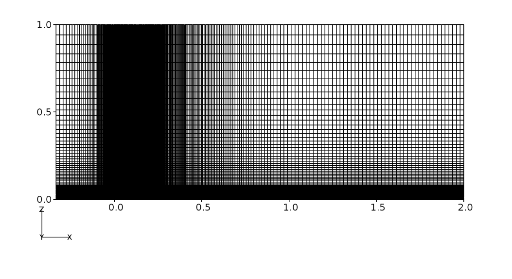
Figure 73 Flat-plate grid (Grid-4) in 2D

Results and Discussion

The steady-state solution of the turbulent flow over a flat plate was obtained using Caelus 9.04. The simpleSolver was used here and the solution was simulated for a sufficient length until the residuals for pressure, velocity and turbulent quantities were less than \(1 \times 10^{-6}\). The finite volume discretization of the gradient of pressure and velocity was carried out using the linear approach. Where as the divergence of velocity and mass flux was carried out through the linear upwind method. However, for the divergence of the turbulent quantities, upwind approach was utilised and linear approach for the divergence of the Reynolds stress terms. For the discretization of the Laplacian terms, again linear corrected method was used. For some grids having greater than 50 degree non-orthogonal angle, linear limited with a value of 0.5 was used for the Laplacian of the turbulent stress terms.

Spalart–Allmaras

In Figure 74, the skin-friction distribution along the flat-plate obtained from Caelus for different grids is shown. As can be seen, all grids produce the same skin-friction values suggesting a grid-independent solution is achieved.

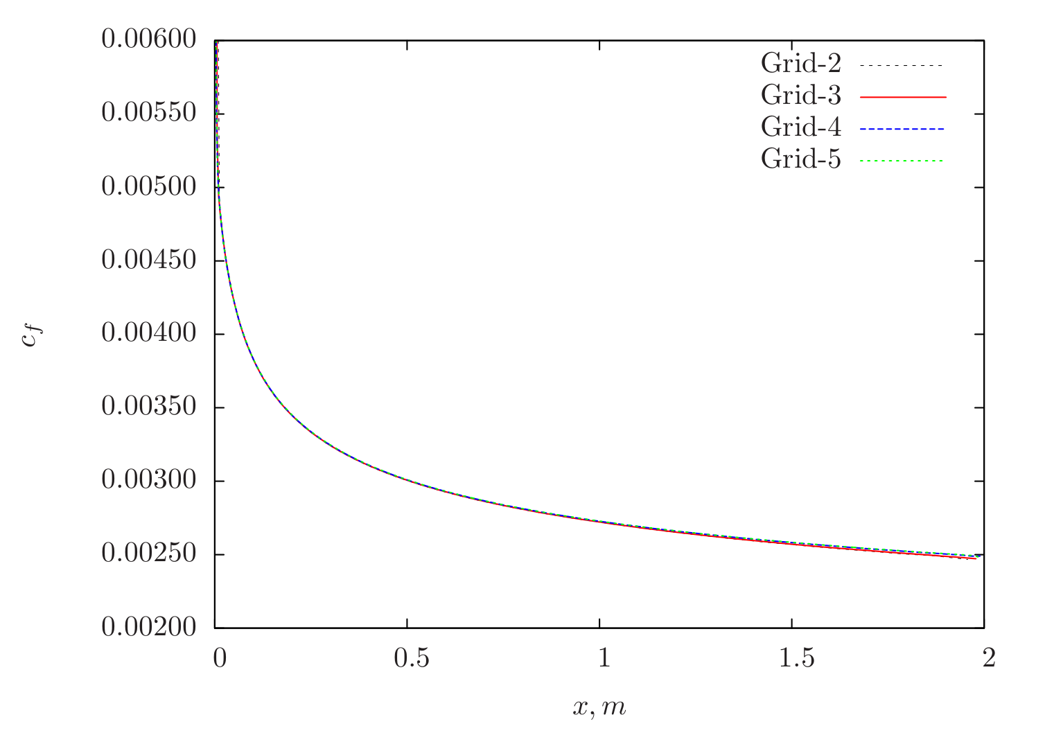
Figure 74 Skin-friction distribution for various grids obtained from Caelus simulation using Spalart–Allmaras turbulence model

In Figure 75, the skin-friction distribution obtained from Caelus on Grid-5 is compared with CFL3D of the same grid. An excellent agreement is obtained all along the plate.

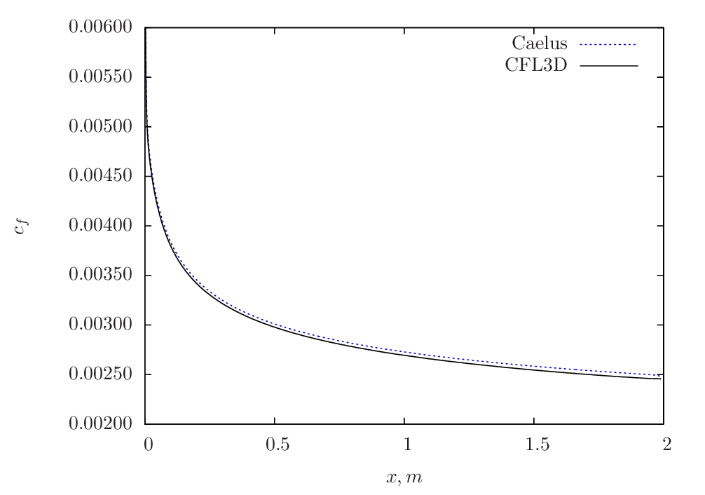
Figure 75 Skin-friction comparison between Caelus and CFL3D using Spalart–Allmaras turbulence model

k-Omega SST

The skin-friction distribution for various grids obtained from \(k-\omega~\rm{SST}\) model is shown in Figure 76.

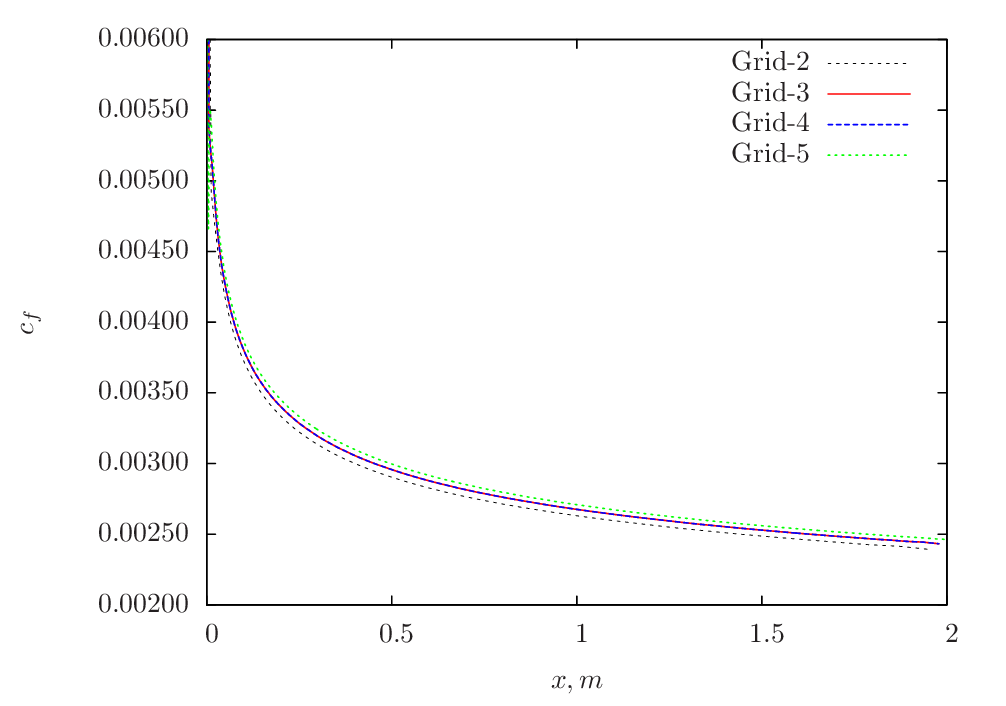
Figure 76 Skin-friction distribution for various grids obtained from Caelus simulation using \(k-\omega~\rm{SST}\) turbulence model

The skin-friction comparison between Caelus and CFL3D for Grid-5 is shown in Figure 77.

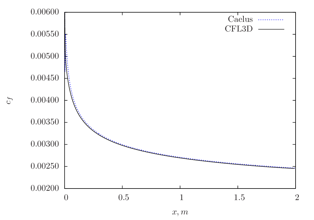
Figure 77 Skin-friction comparison between Caelus and CFL3D using \(k-\omega~\rm{SST}\) turbulence model

Conclusions

The steady turbulent flow over a two-dimensional flat-plate was simulated using Caelus 9.04 utilising the simpleSolver. The simulations were carried out with two turbulence models and the obtained solutions were verified against CFL3D data. The results were found to be in good agreement with CFL3D and suggesting the turbulence implementation in Caelus is accurate.

Two-dimensional Bump in a Channel

Turbulent, incompressible flow over a two-dimensional bump in a channel

Symbol	Definition	Units (SI)
\(a\)	Speed of sound	\(m/s\)
\(c_f\)	Skin friction coefficient	Non-dimensional
\(k\)	Turbulent kinetic energy	\(m^2/s^2\)
\(L\)	Length of the bump	\(m\)
\(M_\infty\)	Freestream Mach number	Non-dimensional
\(p\)	Kinematic pressure	\(Pa/\rho~(m^2/s^2)\)
\(Re_L\)	Reynolds number	\(1/m\)
\(T\)	Temperature	\(K\)
\(u\)	Local velocity in x-direction	\(m/s\)
\(U\)	Freestream velocity in x-direction	\(m/s\)
\(x\)	Distance in x-direction	\(m\)
\(z\)	Distance in z-direction	\(m\)
\(y^+\)	Wall distance	Non-dimensional
\(\mu\)	Dynamic viscosity	\(kg/m~s\)
\(\nu\)	Kinematic viscosity	\(m^2/s\)
\(\tilde{\nu}\)	Turbulence field variable	\(m^2/s\)
\(\rho\)	Density	\(kg/m^3\)
\(\omega\)	Specific dissipation rate	\(1/s\)
\(\infty\)	Freestream conditions
\(t\) (subscript)	Turbulent property

Introduction

This case covers the verification of turbulent incompressible flow over a two-dimensional bump in a channel. The bump acts as a perturbation causing local changes to the velocity and pressure over the bump surface. Since the perturbation is quite small, the flow remains attached to the bump surface. The simulations are carried out over a series of four grids which are successively refined and are studied over two turbulence models, serving as a grid independence study. The distribution of skin-friction (\(c_f\)) is then compared with that of the CFL3D data.

Problem definition

This verification exercise is based on the Turbulence Modeling Resource case for a 2D bump in a channel and follows the same conditions used in the limit of incompressibility. In this case, CFL3D uses a freestream Mach number (\(M_\infty\)) of 0.2. The schematic of the geometric configuration is shown in Figure 78.

Figure 78 Schematic representation of the close-up of the bump (Not to scale)

The location of the plate upstream of the bump begins at x=0 m and ends at x = 1.5 m, giving a total plate length of L = 1.5 m. The flow has a Reynolds number of \(3 \times 10^6\) with a freestream velocity \(U_\infty\) in the x-direction. The temperature of the inflow is assumed to be 300 K and for Air as a perfect gas, the speed of sound (\(a\)) can be evaluated to 347.180 m/s. With the freestream Mach number and speed of sound, the freestream velocity was calculated to \(U_\infty\) = 69.436 m/s. Kinematic viscosity was then obtained from velocity and Reynolds number. The following table summarises the freestream conditions used for this case.

Fluid	\(Re_L~(1/m)\)	\(U_\infty~(m/s)\)	\(p_\infty~(m^2/s^2)\)	\(T_\infty~(K)\)	\(\nu_\infty~(m^2/s)\)
Air	\(3 \times 10^6\)	69.436113	\((0)\) Gauge	300	\(2.314537\times10^{-5}\)

Since the flow is incompressible, the density (\(\rho\)) does not change and therefore, a constant density is assumed throughout the calculation. Further, the temperature is not considered and hence it does not have any influence on viscosity, which is therefore kept constant. Note that in Caelus, pressure and viscosity are always specified as kinematic for a incompressible flow simulation.

Turbulent Properties for Spalart–Allmaras model

The turbulent inflow boundary conditions used for the Spalart–Allmaras model were calculated as \(\tilde{\nu}_{\infty} = 3 \cdot \nu_\infty\) and subsequently turbulent eddy viscosity was evaluated. The following table provides the values of these used in the current simulations:

Table 16 Turbulence freestream conditions for SA model

\(\tilde{\nu}_\infty~(m^2/s)\)	\(\nu_{t~\infty}~(m^2/s)\)
\(6.943611 \times 10^{-5}\)	\(4.8706713 \times 10^{-6}\)

Turbulent Properties for k-omega SST model

The turbulent inflow boundary conditions used for \(k-\omega~\rm{SST}\) were calculated as follows and is as given in Turbulence Modeling Resource

\[k_{\infty} = 9 \times 10^{-9} \cdot a^2_\infty = \frac{0.675 U_\infty}{Re_L}\]

\[\omega_{\infty} = 1 \times 10^{-6} \cdot \frac{\rho_\infty a^2_\infty}{\mu_\infty} = \frac{50 U_\infty}{L}\]

\[\nu_{t~\infty} = 0.009 \times \nu_\infty\]

Note that the dynamic viscosity for the above equation is obtained from Sutherland formulation and density is calculated as \(\rho = \mu / \nu\). The below table provides the turbulent properties used in the current simulations:

Table 17 Turbulence freestream conditions for \(k-\omega~\rm{SST}\) model

\(k_{\infty}~(m^2/s^2)\)	\(\omega_{\infty}~(1/s)\)	\(\nu_{t~\infty}~(m^2/s)\)
\(1.0848 \times 10^{-3}\)	\(5207.6475\)	\(2.08310 \times 10^{-7}\)

Computational Domain and Boundary Conditions

The computational domain consists of a rectangular channel encompassing the bump. In Figure 79 , the details of the boundaries used in two-dimensions (\(x-y\) plane) are shown. The region of interest, which is the bump extends between \(0\leq x \leq 1.5~m\) and has a no-slip boundary condition. Upstream and downstream of the bump, the symmetry boundary extends about 17 bump lengths. The inlet boundary is placed at the start of the symmetry at \(x = -25.0~m\) and the outlet is placed at \(x = 26.5~m\). For the entire top boundary, symmetry plane condition is used.

Figure 79 Computational domain for a 2D bump (Not to scale)

Boundary Conditions and Initialisation

Following are the boundary condition details used for the computational domain:

• Inlet

  • Velocity: Fixed uniform velocity \(u = 69.436113~m/s\) in \(x\) direction

  • Pressure: Zero gradient

  • Turbulence:

    • Spalart–Allmaras (Fixed uniform values of \(\nu_{t~\infty}\) and \(\tilde{\nu}_{\infty}\) as given in the above table)

    • \(k-\omega~\rm{SST}\) (Fixed uniform values of \(k_{\infty}\), \(\omega_{\infty}\) and \(\nu_{t~\infty}\) as given in the above table)

• Symmetry

  • Velocity: Symmetry

  • Pressure: Symmetry

  • Turbulence: Symmetry

• No-slip wall

  • Velocity: Fixed uniform velocity \(u, v, w = 0\)

  • Pressure: Zero gradient

  • Turbulence:

    • Spalart–Allmaras (Fixed uniform values of \(\nu_{t}=0\) and \(\tilde{\nu}=0\))

    • \(k-\omega~\rm{SST}\) (Fixed uniform values of \(k = 0\) and \(\nu_t=0\); \(\omega\) = omegaWallFunction)

• Outlet

  • Velocity: Zero gradient velocity

  • Pressure: Fixed uniform gauge pressure \(p = 0\)

  • Turbulence:

    • Spalart–Allmaras (Calculated \(\nu_{t}=0\) and Zero gradient \(\tilde{\nu}\))

    • \(k-\omega~\rm{SST}\) (Zero gradient \(k\) and \(\omega\); Calculated \(\nu_t=0\); )

• Initialisation

  • Velocity: Fixed uniform velocity \(u = 69.436113~m/s\) in \(x\) direction

  • Pressure: Zero Gauge pressure

  • Turbulence:

    • Spalart–Allmaras (Fixed uniform values of \(\nu_{t~\infty}\) and \(\tilde{\nu}_{\infty}\) as given in the above table)

    • \(k-\omega~\rm{SST}\) (Fixed uniform values of \(k_{\infty}\), \(\omega_{\infty}\) and \(\nu_{t~\infty}\) as given in the above table)

Computational Grid

The 3D computational grid was obtained from Turbulence Modeling Resource as a Plot3D and was converted to Caelus format using Pointwise. In the Plot3D computational grid, the flow normal direction is \(z\) and thus the two-dimensional plane of interest is in \(x-z\) directions. Further, since the flow-field is of two-dimensional, and the simpleSolver being a 3D solver, the two \(x-z\) planes are specified with empty boundary conditions. A series of four grids were considered from the original set of five, excluding the coarsest grid and the following table give its details.

Grid	Cells in \(x\)-direction	Cells in \(z\)-direction	Total	\(y^+\)
Grid-2	176	80	14,080	0.236
Grid-3	352	160	56,320	0.118
Grid-4	704	320	225,280	0.059
Grid-5	1408	640	901,120	0.03

The 2D grid in \(x-z\) plane is shown in Figure 80 for Grid-3. As can be noted, the grid is sufficiently refined close to the wall in the normal direction. In addition, the grids are refined in the vicinity of the bump, including both upstream and downstream which can be seen in the inset. All grids have a \(y^+ < 1\) and no wall function is used for the wall boundary in the current verification cases.

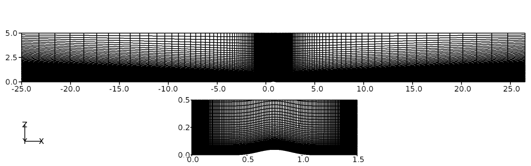
Figure 80 Bump grid (Grid-3) in 2D

Results and Discussion

The steady-state solution of the turbulent flow over a two-dimensional bump was obtained using Caelus 9.04. The simpleSolver was used for the calculations and was run for a sufficient length until the residuals for pressure, velocity and turbulent quantities were less than \(1 \times 10^{-6}\). The finite volume discretization of the gradient of pressure and velocity was carried out using the linear approach. Where as the divergence of velocity and mass flux was carried out through the linear upwind method. However, for the divergence of the turbulent quantities, upwind approach was utilised and linear approach for the divergence of the Reynolds stress terms. For the discretization of the Laplacian terms, again linear corrected method was used. For some grids having greater than 50 degree non-orthogonal angle, linear limited with a value of 0.5 was used for the Laplacian of the turbulent stress terms.

Spalart–Allmaras

The skin-friction distributions over the 2D bump obtained from Caelus for different grids are shown in Figure 81. There is very little difference in the skin-friction beyond Grid-2 suggesting that a grid-independence solution is achieved.

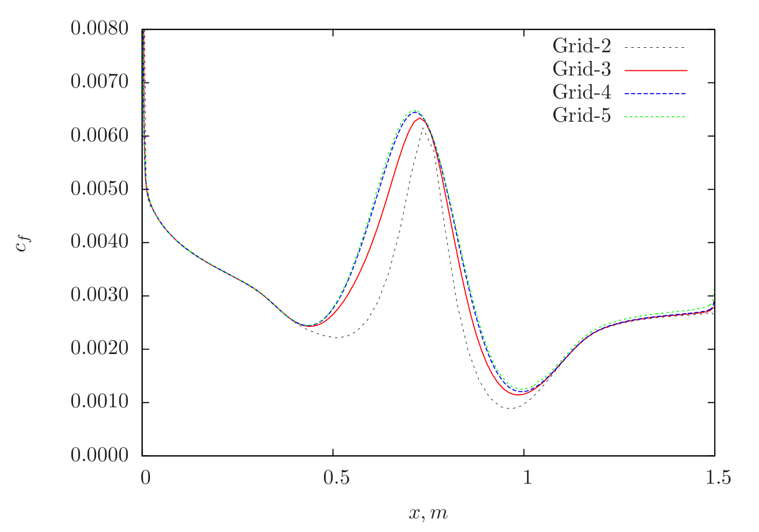
Figure 81 Skin-friction distribution for various grids obtained from Caelus simulation using Spalart–Allmaras turbulence model

In Figure 82 , the comparison between Caelus and CFL3D is made for Grid-5 and as can be seen, a very good agreement is obtained over the entire region of the bump.

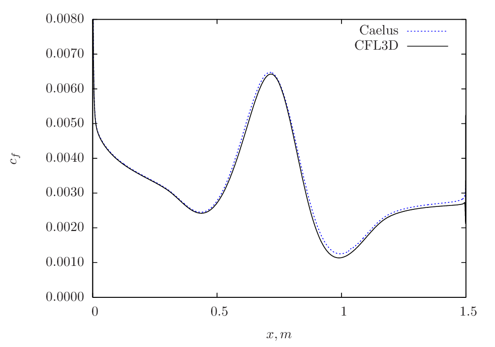
Figure 82 Skin-friction comparison between Caelus and CFL3D using Spalart–Allmaras turbulence model

k-Omega SST

The skin-friction distribution variation for different grids obtained from \(k-\omega~\rm{SST}\) model is shown in Figure 83.

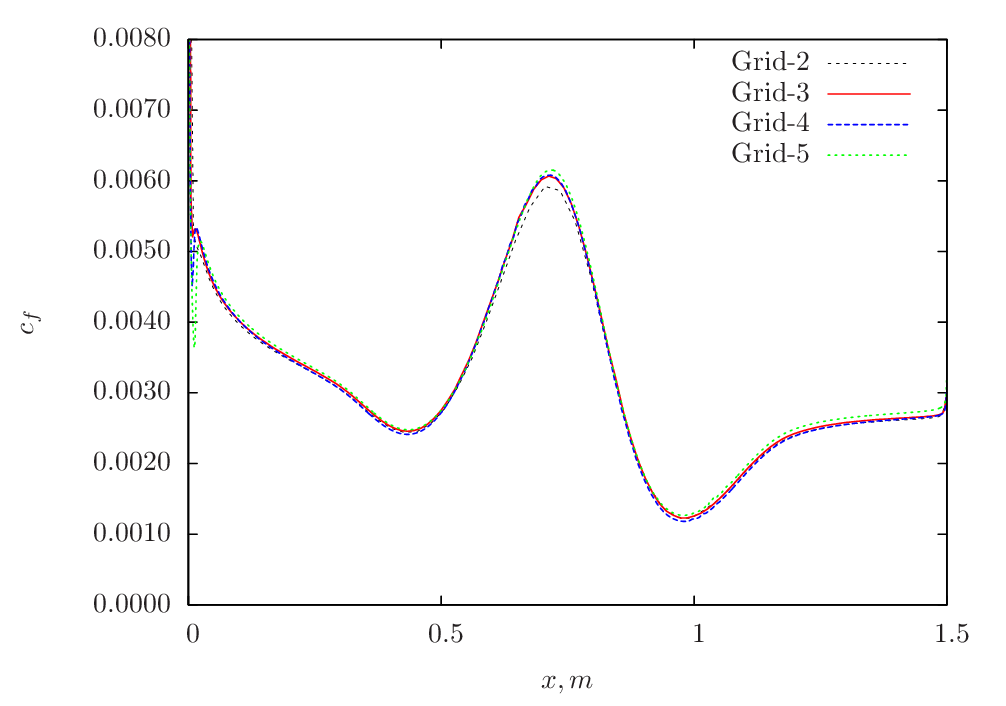
Figure 83 Skin-friction distribution for various grids obtained from Caelus simulation using \(k-\omega~\rm{SST}\) turbulence model

In Figure 84 , the skin-friction comparison between Caelus and CFL3D is made for Grid-5 and is shown.

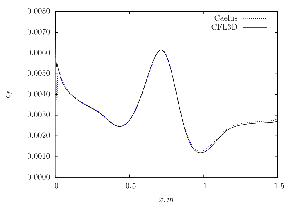
Figure 84 Skin-friction comparison between Caelus and CFL3D using \(k-\omega~\rm{SST}\) turbulence model

Conclusions

The steady turbulent flow simulation over a two-dimensional bump was carried out using Caelus 9.04 employing simpleSolver. The solutions were obtained with two turbulence models, implemented in-house and the results were verified against CFL3D data. The comparison was found to be in good agreement with CFL3D suggesting that the turbulence model implementation is accurate in Caelus.

Two-dimensional NACA 0012 Airfoil

Nomenclature

Turbulent, incompressible flow over a two-dimensional NACA airfoil

Symbol	Definition	Units (SI)
\(a\)	Speed of sound	\(m/s\)
\(c_f\)	Skin friction coefficient	Non-dimensional
\(c_p\)	Pressure coefficient	Non-dimensional
\(C\)	Chord length	\(m\)
\(I\)	Turbulent intensity	Percentage
\(k\)	Turbulent kinetic energy	\(m^2/s^2\)
\(M_\infty\)	Freestream Mach number	Non-dimensional
\(p\)	Kinematic pressure	\(Pa/\rho~(m^2/s^2)\)
\(Re_L\)	Reynolds number	\(1/m\)
\(T\)	Temperature	\(K\)
\(u\)	Local velocity in x-direction	\(m/s\)
\(w\)	Local velocity in z-direction	\(m/s\)
\(U\)	Freestream velocity	\(m/s\)
\(x\)	Distance in x-direction	\(m\)
\(z\)	Distance in y-direction	\(m\)
\(y^+\)	Wall distance	Non-dimensional
\(\alpha\)	Angle of attack	Degrees
\(\mu\)	Dynamic viscosity	\(kg/m~s\)
\(\nu\)	Kinematic viscosity	\(m^2/s\)
\(\tilde{\nu}\)	Turbulence field variable	\(m^2/s\)
\(\rho\)	Density	\(kg/m^3\)
\(\omega\)	Specific dissipation rate	\(1/s\)
\(\infty\)	Freestream conditions
\(t\) (subscript)	Turbulent property

Introduction

This case deals with the steady turbulent incompressible flow over a two-dimensional NACA 0012 airfoil. The study is conducted at two angles of attack, \(\alpha = 0^\circ\) and \(\alpha = 10^\circ\) respectively. The simulations are carried out over a series of four grids and compared with CFL3D data and the results are also compared with the experimental data. This exercise therefore verifies and validates the turbulence models used through the distribution of skin-friction coefficient (\(c_f\)) and pressure coefficient (\(c_p\)) over the airfoil surface.

Problem definition

This verification and validation exercise is based on the Turbulence Modeling Resource case for a NACA 0012 airfoil and follows the same flow conditions used in the incompressible limit. However, the numerical code CFL3D uses a freestream Mach number (\(M_\infty\)) of 0.15. In Figure 85 the schematic of the airfoil is shown. Note that the 2D plane in Figure 85 is depicted in \(x-z\) directions as the computational grid also follows the same 2D plane.

Figure 85 Schematic representation of the 2D airfoil (Not to scale)

The length of the airfoil chord is C = 1.0 m, wherein, x = 0 is at the leading edge and the Reynolds number is \(6 \times 10^6\) and \(U_\infty\) is the freestream velocity. For \(\alpha = 10^\circ\), the velocity components are evaluated in order to have a same resultant freestream velocity. The freestream flow temperature in this case is assumed to be 300 K and for Air as a perfect gas, the speed of sound (\(a\)) can be evaluated to 347.180 m/s. Based on the freestream Mach number and speed of sound, freestream velocity can be evaluated to \(U_\infty\) = 52.077 m/s. Using the value of velocity and Reynolds number, kinematic viscosity can be calculated. The following table summarises the freestream conditions used:

Fluid	\(Re_L~(1/m)\)	\(U_\infty~(m/s)\)	\(p_\infty~(m^2/s^2)\)	\(T_\infty~(K)\)	\(\nu_\infty~(m^2/s)\)
Air	\(6 \times 10^6\)	52.0770	\((0)\) Gauge	300	\(8.679514\times10^{-6}\)

To get a freestream velocity of \(U_\infty\) = 52.077 m/s at \(\alpha = 10^\circ\), the velocity components in \(x\) and \(z\) are resolved. These are provided in the table below

\(\alpha~\rm{(Degrees)}\)	\(u~(m/s)\)	\(w~(m/s)\)
\(0^\circ\)	52.0770	0.0
\(10^\circ\)	51.2858	9.04307

Note that in an incompressible flow, the density (\(\rho\)) does not vary and a constant density can be assumed throughout the calculation. Further, since temperature is not considered here, the viscosity is also held constant. In Caelus for incompressible flow simulations, pressure and viscosity are always specified as kinematic.

Turbulent Properties for Spalart–Allmaras model

The turbulent inflow boundary conditions used for the Spalart–Allmaras model were calculated as \(\tilde{\nu}_{\infty} = 3 \cdot \nu_\infty\) and subsequently turbulent eddy viscosity was evaluated. The following table provides the values of these used in the current simulations:

Table 18 Turbulent freestream conditions for SA Model

\(\tilde{\nu}_\infty~(m^2/s)\)	\(\nu_{t~\infty}~(m^2/s)\)
\(2.603854 \times 10^{-5}\)	\(1.8265016 \times 10^{-6}\)

Turbulent Properties for k-omega SST model

The turbulent inflow boundary conditions used for \(k-\omega~\rm{SST}\) were calculated as follows and is as given in Turbulence Modeling Resource

\[k_{\infty} = \frac{3}{2} (U_\infty I)^2\]

\[\omega_{\infty} = 1 \times 10^{-6} \cdot \frac{\rho_\infty a^2_\infty}{\mu_\infty} = \frac{266.7 U_\infty}{L}\]

\[\nu_{t~\infty} = 0.009 \times \nu_\infty\]

Note that the dynamic viscosity in the above equation is obtained from Sutherland formulation and density is evaluated as \(\rho = \mu / \nu\). In the below table, the turbulent properties used in the current simulations are provided.

Table 19 Turbulent freestream conditions for SST Model

\(I\)	\(k_{\infty}~(m^2/s^2)\)	\(\omega_{\infty}~(1/s)\)	\(\nu_{t~\infty}~(m^2/s)\)
\(0.052\%\)	\(1.0999 \times 10^{-3}\)	\(13887.219\)	\(7.811564 \times 10^{-8}\)

Computational Domain and Boundary Conditions

The computational domain used for the airfoil simulations and the details of the boundaries are shown in Figure 86 for a \(x-z\) plane. The leading edge and the trailing edge extends between \(0 \leq x \leq 1.0~m\) and the entire airfoil has a no-slip boundary condition. The far-field domain extends by about 500 chord lengths in the radial direction and the inlet is placed for the entire boundary highlighted in green. The outlet boundary is placed at the exit plane, which is at \(x \approx 500~m\).

Figure 86 Computational domain for a 2D airfoil (Not to scale)

Boundary Conditions and Initialisation

• Inlet

  • Velocity:

    • \(\alpha=0^\circ\): Fixed uniform velocity \(u = 52.0770~m/s\); \(v = w = 0.0~m/s\) in \(x, y\) and \(z\) directions respectively

    • \(\alpha=10^\circ\): Fixed uniform velocity \(u = 51.2858~m/s\); \(v = 0.0~m/s\) and \(w = 9.04307~m/s\) in \(x, y\) and \(z\) directions respectively

    • Pressure: Zero gradient

    • Turbulence:

      • Spalart–Allmaras (Fixed uniform values of \(\nu_{t~\infty}\) and \(\tilde{\nu}_{\infty}\) as given in the above table)

      • \(k-\omega~\rm{SST}\) (Fixed uniform values of \(k_{\infty}\), \(\omega_{\infty}\) and \(\nu_{t~\infty}\) as given in the above table)

• No-slip wall

  • Velocity: Fixed uniform velocity \(u, v, w = 0\)

  • Pressure: Zero gradient

  • Turbulence:

    • Spalart–Allmaras (Fixed uniform values of \(\nu_{t}=0\) and \(\tilde{\nu}=0\))

    • \(k-\omega~\rm{SST}\) (Fixed uniform values of \(k = <<0\) and \(\nu_t=0\); \(\omega\) = omegaWallFunction)

• Outlet

  • Velocity: Zero gradient velocity

  • Pressure: Fixed uniform gauge pressure \(p = 0\)

  • Turbulence:

    • Spalart–Allmaras (Calculated \(\nu_{t}=0\) and Zero gradient \(\tilde{\nu}\))

    • \(k-\omega~\rm{SST}\) (Zero gradient \(k\) and \(\omega\); Calculated \(\nu_t=0\); )

• Initialisation

  • Velocity:

    • \(\alpha=0^\circ\): Fixed uniform velocity \(u = 52.0770~m/s\); \(v = w = 0.0~m/s\) in \(x, y\) and \(z\) directions respectively

    • \(\alpha=10^\circ\): Fixed uniform velocity \(u = 51.2858~m/s\); \(v = 0.0~m/s\) and \(w = 9.04307~m/s\) in \(x, y\) and \(z\) directions respectively

    • Pressure: Zero Gauge pressure

    • Turbulence:

      • Spalart–Allmaras (Fixed uniform values of \(\nu_{t~\infty}\) and \(\tilde{\nu}_{\infty}\) as given in the above table)

      • \(k-\omega~\rm{SST}\) (Fixed uniform values of \(k_{\infty}\), \(\omega_{\infty}\) and \(\nu_{t~\infty}\) as given in the above table)

Computational Grid

The 3D computational grid for the NACA 0012 airfoil was obtained from Turbulence Modeling Resource as a Plot3D format. Using Pointwise it was then converted to Caelus format. As indicated earlier, the two-dimensional plane of interest in the Plot3D grid is in \(x-z\) directions. As the flow is considered here to be two-dimensional, and simpleSolver being a 3D solver, the two \(x-z\) planes are specified with empty boundary conditions consequently treating as symmetry flow in \(y\) direction. To study the sensitivity of the grid, four grids were considered from the original set of five, in which the coarsest grid was excluded from this study. Details of the different grids used are given in the below table. Not that for both angles of attack, same grid is used.

Grid	Cells over airfoil	Cells in normal direction	Total	\(y^+\)
Grid-2	128	64	14,336	0.465
Grid-3	256	128	57,344	0.209
Grid-4	512	256	229,376	0.098
Grid-5	1024	512	917,504	0.047

The below Figure 87 shows the 2D grid in \(x-z\) plane for Grid-3 and the refinement around the airfoil is shown in the inset. Sufficient refinement can be seen in the wall normal direction and all the grid have a \(y^+ < 1\) and no wall function is used for the airfoil surface throughout the current verification and validation cases.

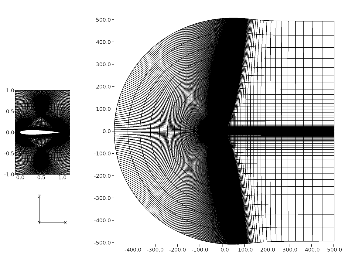
Figure 87 Airfoil grid (Grid-3) shown in 2D

Results and Discussion

The solution to the turbulent flow over the NACA 0012 airfoil was obtained using Caelus 9.04. SimpleSolver was used and the solutions were run sufficiently long until the residuals for pressure, velocity and turbulence quantities were less than \(1 \times 10^{-6}\). The finite volume discretization of the gradient of pressure and velocity was carried out using the linear approach. Where as the divergence of velocity and mass flux was carried out through the linear upwind method. However, for the divergence of the turbulent quantities, upwind approach was utilised and linear approach for the divergence of the Reynolds stress terms. For the discretization of the Laplacian terms, again linear corrected method was used. For some grids having greater than 50 degree non-orthogonal angle, linear limited with a value of 0.5 was used for the Laplacian of the turbulent stress terms.

The verification results are shown firstly for both angles of attack and is followed by the experimental validation data.

Verification results: Spalart–Allmaras

The following Figure 88 and Figure 89 shows the skin-friction distribution over the upper surface for \(\alpha=0^\circ\) and \(\alpha=10^\circ\) from Caelus for different grids. In both cases, Grid-4 and Grid-5 essentially produces the same solution suggesting a grid-independence solution is obtained.

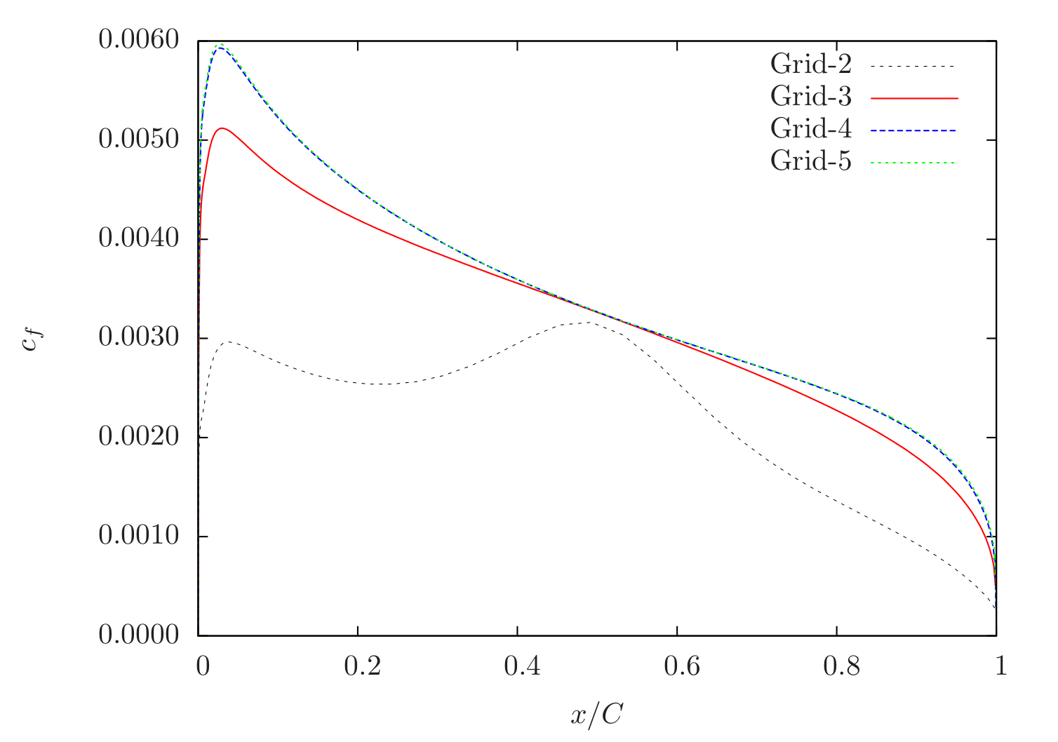
Figure 88 Skin-friction distribution obtained from Caelus simulations using SA turbulence model for \(\alpha=0^\circ\)

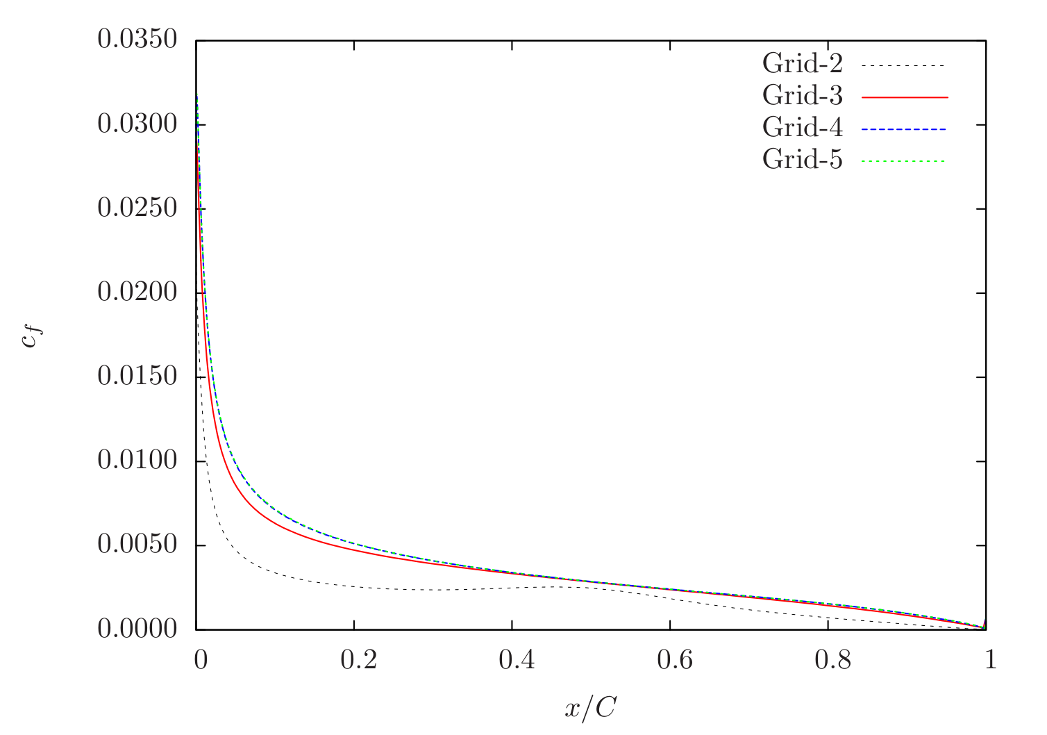
Figure 89 Skin-friction distribution obtained from Caelus simulations using SA turbulence model for \(\alpha=10^\circ\)

In Figure 90 and Fig. #turbulent-airfoil-caelus-cfl3d-sacc-10 , the skin-friction is compared with CFL3D on Grid-4. As can be seen, a very good agreement between the two codes can be seen.

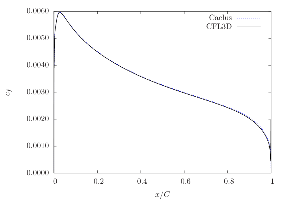
Figure 90 Skin-friction comparison between Caelus and CFL3D using SA turbulence model for \(\alpha=0^\circ\)

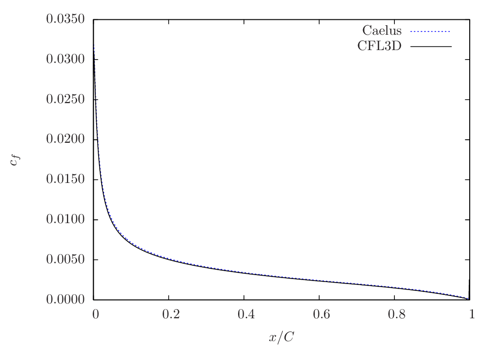
Figure 91 Skin-friction comparison between Caelus and CFL3D using SA turbulence model for \(\alpha=10^\circ\)

Verification results: k-omega SST

The skin-friction distribution obtained from using \(k-\omega~\rm{SST}\) turbulence model for \(\alpha=0^\circ\) and \(\alpha=10^\circ\) is shown below for different grids. The grid-sensitivity behaviour is very similar to the Spalart–Allmaras turbulence case and no change is seen between Grid-4 and Grid-5.

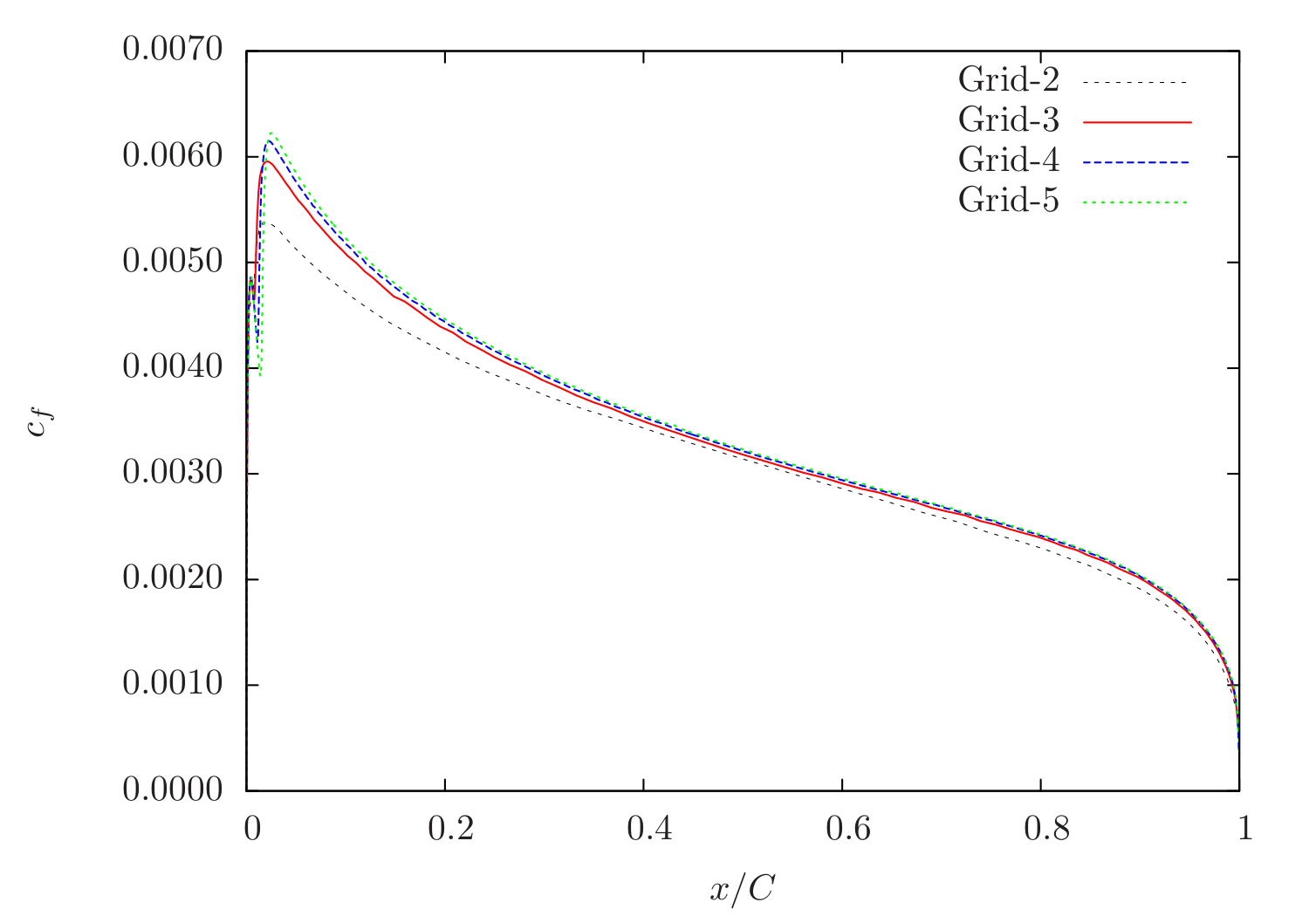
Figure 92 Skin-friction distribution obtained from Caelus simulations using \(k-\omega~\rm{SST}\) turbulence model for \(\alpha=0^\circ\)

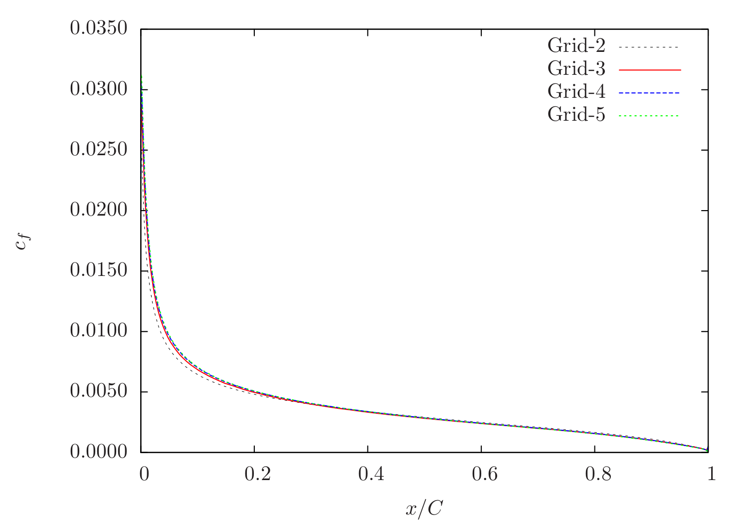
Figure 93 Skin-friction distribution obtained from Caelus simulations using \(k-\omega~\rm{SST}\) turbulence model for \(\alpha=10^\circ\)

The comparison of the skin-friction with CFL3D using \(k-\omega~\rm{SST}\) is shown in Figure 94 and Figure 95 for both angle of attacks and similar to the previous case, a very good agreement between the two can be seen.

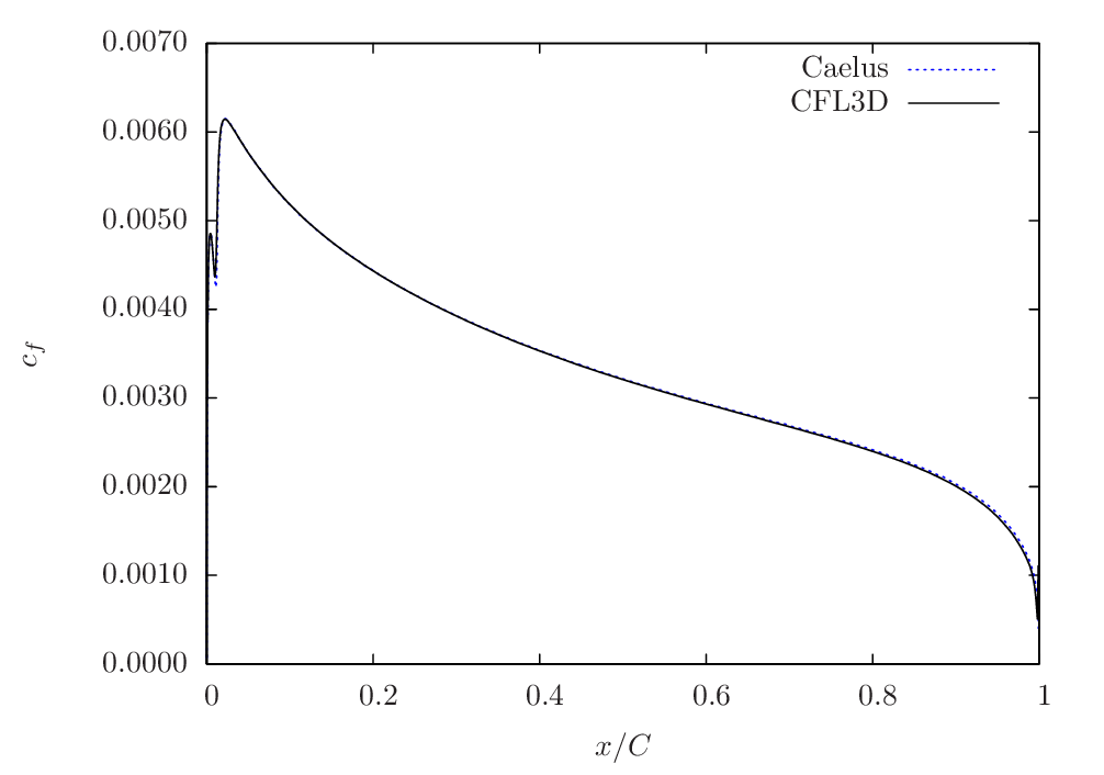
Figure 94 Skin-friction comparison between Caelus and CFL3D using \(k-\omega~\rm{SST}\) turbulence model for \(\alpha=0^\circ\)

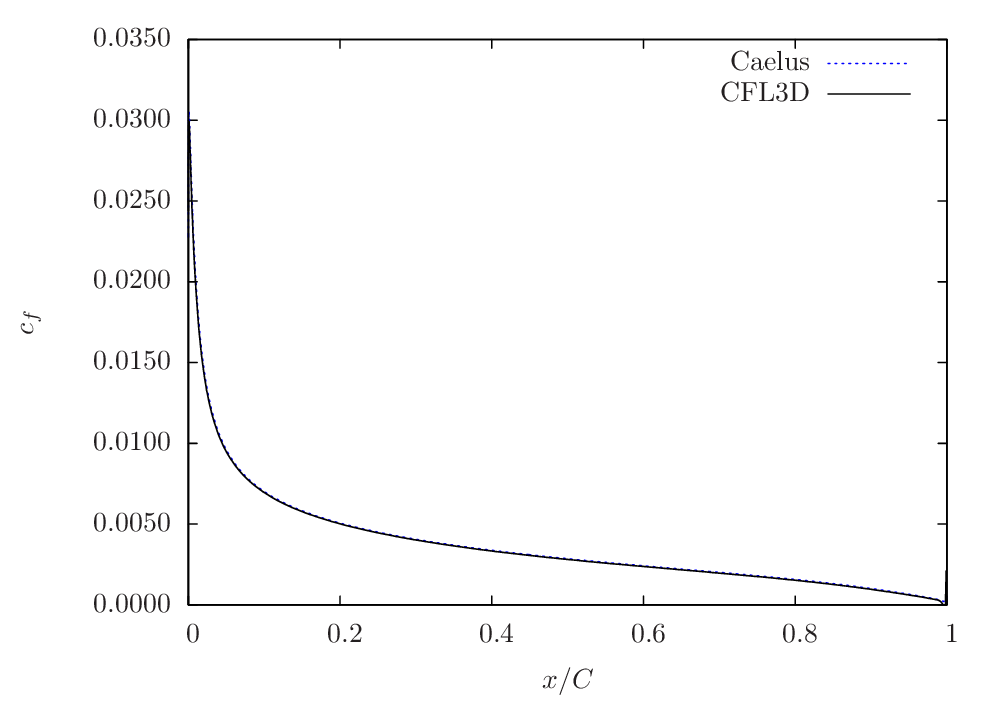
Figure 95 Skin-friction comparison between Caelus and CFL3D using \(k-\omega~\rm{SST}\) turbulence model for \(\alpha=10^\circ\)

Experimental validation

Here, the Caelus data is compared with the pressure-coefficient (\(c_p\)) obtained experimentally by Gregory, N. and O’Reilly, C. L [5] for both angles of attack over the upper surface. In addition, the data obtained from CFL3D is also included for verification. There is a very good agreement with the current Caelus and experiments which indicates that the correct turbulence equations are being solved in both Spalart–Allmaras and \(k-\omega~\rm{SST}\) models.

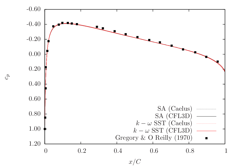
Figure 96 Pressure comparison between Caelus, experiments and CFL3D for \(\alpha=0^\circ\)

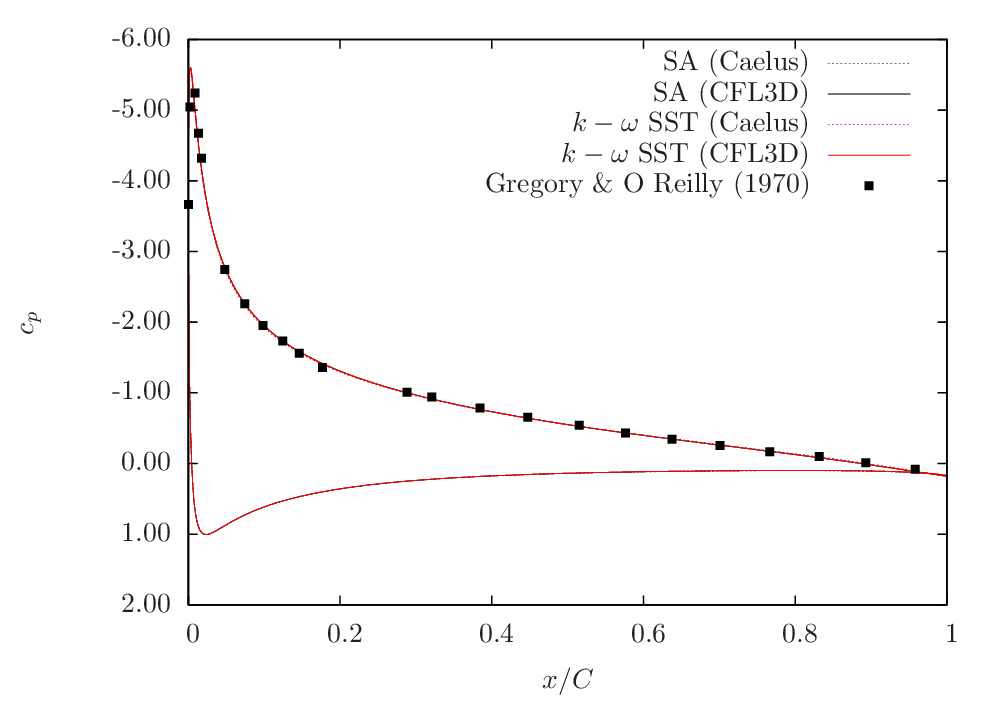
Figure 97 Pressure comparison between Caelus, experiments and CFL3D for \(\alpha=10^\circ\)

Conclusions

Verification and validation over a two-dimensional NACA 0012 airfoil for turbulent inflow conditions were carried out using Caelus 9.04 employing simpleSolver. Two turbulence models that are implemented in-house were used and the solutions were verified with CFL3D data and subsequently validated with the experimental pressure coefficient values. The results were found to be in very good agreement suggesting that the turbulence modelling implementation is appropriate and solves accurately.

Two-dimensional Convex Curvature

Turbulent, incompressible flow in a two-dimensional convex curvature channel

Nomenclature

Symbol	Definition	Units (SI)
\(a\)	Speed of sound	\(m/s\)
\(c_f\)	Skin friction coefficient	Non-dimensional
\(c_p\)	Pressure coefficient	Non-dimensional
\(I\)	Turbulent intensity	Percentage
\(k\)	Turbulent kinetic energy	\(m^2/s^2\)
\(M_i\)	Inlet Mach number	Non-dimensional
\(p\)	Kinematic pressure	\(Pa/\rho~(m^2/s^2)\)
\(Re_L\)	Reynolds number	\(1/m\)
\(T\)	Temperature	\(K\)
\(u\)	Local velocity in x-direction	\(m/s\)
\(w\)	Local velocity in z-direction	\(m/s\)
\(U\)	Inlet velocity	\(m/s\)
\(x\)	Distance in x-direction	\(m\)
\(y\)	Distance in y-direction	\(m\)
\(y^+\)	Wall distance	Non-dimensional
\(\alpha\)	Angle of attack	Degrees
\(\mu\)	Dynamic viscosity	\(kg/m~s\)
\(\nu\)	Kinematic viscosity	\(m^2/s\)
\(\tilde{\nu}\)	Turbulence field variable	\(m^2/s\)
\(\rho\)	Density	\(kg/m^3\)
\(\omega\)	Specific dissipation rate	\(1/s\)
\(i\)	Inlet conditions
\(t\) (subscript)	Turbulent property
\(ref\)	Reference pressure	\(Pa\)

Introduction

In this case, the turbulent incompressible flow in a constant-area duct having a convex curvature is investigated as a part of verification and validation. The effect of curvature on the capability of turbulence model to predict the boundary layer accurately is of primary concern in this study. Similar to previous cases, the simulations are carried out over a series of four grids that tests the sensitivity of solution as the grid is refined. As with the earlier cases, Spalart-Allmaras (SA) and \(k-\omega~\rm{SST}\) turbulence models are tested. However due to the presence of strong curvature, a variant of Spalart–Allmaras turbulence model which accounts for rotational and curvature effects is additionally considered. This model is referred to as “Spalart–Allmaras Rotational/Curvature” (SA-RC) [9] . The results are then verified against CFL3D data and validated with experimental pressure distributions.

Problem definition

This verification and validation exercise is based on the Turbulence Modeling Resource case and follows the same conditions used in the incompressible limit. As CFL3D is a compressible CFD code, the original simulation used a inlet Mach number (\(M_i\)) of 0.093. A schematic of the geometric configuration is shown below and is depicted in \(x-z\) plane as the computational grid also follows the same 2D plane of flow.

Figure 98 Schematic representation of the 2D curvature geometry (Not to scale)

As can be seen above, the 2D duct has a rapid bend of \(\alpha = 30^\circ\) after about a distance of 1.4 m and the downstream extends up to 1.6 m in length. The cross-section of the duct is 0.127 m and the inner radius and outer radius of curvature are 0.127 m and 0.254 m respectively. The flow has a Reynolds number of \(2.1 \times 10^6\) and U is the inlet velocity. To achieve a desired inlet velocity at an angle of 30 degrees, the velocity components are evaluated. The inlet temperature for this case is T = 293 K and for Air as a perfect gas, the speed of sound (\(a\)) can be evaluated to 343.106 m/s. Based on the inlet Mach number and speed of sound, the inlet velocity can be calculated to U = 31.908 m/s. Using velocity and Reynolds number kinematic viscosity can be calculated. The table below summarises the inlet conditions used:

Fluid	\(Re_L~(1/m)\)	\(U~(m/s)\)	\(p~(m^2/s^2)\)	\(T~~(K)\)	\(\nu_i~(m^2/s)\)
Air	\(2.1 \times 10^6\)	31.9088	\((0)\) Gauge	293	\(1.519470\times10^{-5}\)

In order to achieve a inlet velocity of U = 31.9088 m/s at \(\alpha=30^\circ\), the velocity components in \(x\) and \(z\) are resolved. These are given below

\(\alpha~\rm{(Degrees)}\)	\(u~(m/s)\)	\(w~(m/s)\)
\(30^\circ\)	27.63389	15.95443

It should be noted that in an incompressible flow, the density (\(\rho\)) does not vary and a constant density assumption is valid throughout the calculation. Further, the temperature field is not solved and therefore its influence on viscosity can be neglected and a constant viscosity can be used. In Caelus for incompressible flow simulations, pressure and viscosity are always specified as kinematic.

Turbulent Properties for Spalart–Allmaras and Spalart–Allmaras Curvature Correction model

The inflow conditions used for turbulent properties in Spalart-Allamaras model was calculated as \(\tilde{\nu}_{i} = 3 \cdot \nu_i\) and subsequently turbulent eddy viscosity was evaluated. The following table provides the values of these used in the current simulations:

Table 20 Turbulent freestream conditions for SA Model

\(\tilde{\nu}_i~(m^2/s)\)	\(\nu_{t~i}~(m^2/s)\)
\(4.558411 \times 10^{-5}\)	\(3.197543 \times 10^{-6}\)

Turbulent Properties for k-omega SST model

The turbulent inflow boundary conditions used for \(k-\omega~\rm{SST}\) were calculated as follows and is as given in Turbulence Modeling Resource

\[k_{i} = \frac{3}{2} (U_i I)^2\]

\[\omega_{i} = 1 \times 10^{-6} \cdot \frac{\rho_i a^2_i}{\mu_i}\]

\[\nu_{t~i} = 0.009 \times \nu_i\]

Note that the dynamic viscosity in the above equation is obtained from Sutherland formulation and density is evaluated as \(\rho = \mu / \nu\). In the below table, the turbulent properties used in the current simulations are provided

Table 21 Turbulent freestream conditions for SST Model

\(I\)	\(k_{i}~(m^2/s^2)\)	\(\omega_{i}~(1/s)\)	\(\nu_{t~i}~(m^2/s)\)
\(0.083\%\)	\(1.0521 \times 10^{-3}\)	\(7747.333\)	\(1.36756 \times 10^{-7}\)

Computational Domain and Boundary Conditions

The computational domain for the duct is quite simple and follows the geometry as is shown in Figure 99. The walls are modelled as no-slip boundary and is highlighted in blue and the outlet is placed at the end of the duct.

Figure 99 Computational domain for a 2D convex curvature (Not to scale)

Boundary Conditions and Initialisation

• Inlet

  • Velocity: Fixed uniform velocity \(u = 27.63389~m/s\); \(v = 0.0~m/s\) and \(w = 15.95443~m/s\) in \(x, y\) and \(z\) directions respectively

  • Pressure: Zero gradient

  • Turbulence:

    • SA & SA-RC (Fixed uniform values of \(\nu_{t~i}\) and \(\tilde{\nu}_{i}\) as given in the above table)

    • \(k-\omega~\rm{SST}\) (Fixed uniform values of \(k_{i}\), \(\omega_{i}\) and \(\nu_{t~i}\) as given in the above table)

• No-slip wall

  • Velocity: Fixed uniform velocity \(u, v, w = 0\)

  • Pressure: Zero gradient

  • Turbulence:

    • SA & SA-RC (Fixed uniform values of \(\nu_{t}=0\) and \(\tilde{\nu} =0\))

    • \(k-\omega~\rm{SST}\) (Fixed uniform values of \(k = 0\) and \(\nu_t=0\); \(\omega\) = omegaWallFunction)

• Outlet

  • Velocity: Zero gradient velocity

  • Pressure: Fixed uniform gauge pressure \(p = 0\)

  • Turbulence:

    • SA & SA-RC (Calculated \(\nu_{t}=0\) and Zero gradient \(\tilde{\nu}\))

    • \(k-\omega~\rm{SST}\) (Zero gradient \(k\) and \(\omega\); Calculated \(\nu_t=0\); )

• Initialisation

  • Velocity: Fixed uniform velocity \(u = 27.63389~m/s\); \(v = 0.0~m/s\) and \(w = 15.95443~m/s\) in \(x, y\) and \(z\) directions respectively

  • Pressure: Zero Gauge pressure

  • Turbulence:

    • SA & SA-RC (Fixed uniform values of \(\nu_{t~i}\) and \(\tilde{\nu}_{i}\) as given in the above table)

    • \(k-\omega~\rm{SST}\) (Fixed uniform values of \(k_{i}\), \(\omega_{i}\) and \(\nu_{t~i}\) as given in the above table)

Computational Grid

The computational grid in 3D for the convex curvature duct was obtained from Turbulence Modeling Resource as a Plot3D format. The same was used in Caelus by converting it in the required format with the use of Pointwise. Since the flow field is assumed to the two-dimensional, the 2D computational plane of interest is in \(x-z\) directions. SimpleSolver is a 3D solver, therefore the two additional \(x-z\) planes are specified with empty boundary conditions. To look at the effect of grid sensitivity, four grids were considered from the original set of five, while the coarsest grid was not included in this study. The table below gives the details of different grids used.

Grid	Cells in streamwise direction	Cells in normal direction	Total
Grid-2	128	48	6144
Grid-3	256	96	98304
Grid-4	512	192	98,304
Grid-5	1024	384	393,216

The 2D convex curvature grid is shown in Figure 100 below, for Grid-3 in \(x-z\) plane and the inset shows the grids in the vicinity of the strong curvature. Grids are refined close to the wall in order to capture the turbulent boundary layer and all grids have a \(y^+ < 1\) and no wall function is used through the validation and verification of this configuration.

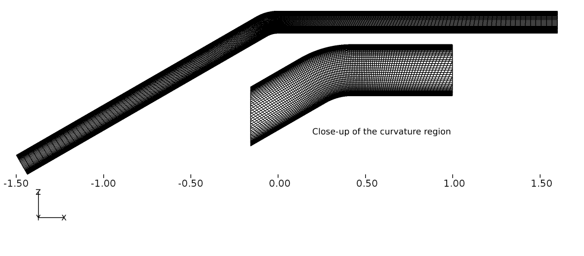
Figure 100 Convex curvature grid (Grid-3) shown in 2D (Inset shows the close-up of the curvature region)

Results and Discussion

The turbulent flow inside the convex curvature duct was simulated using Caelus 9.04 through the use of simpleSolver. The solutions were run until the residuals for pressure, velocity and turbulent quantities were less than \(1 \times 10^{-6}\). The finite volume discretization of the gradient of pressure and velocity was carried out using the linear approach. Where as the divergence of velocity and mass flux was carried out through the linear upwind method. However, for the divergence of the turbulent quantities, upwind approach was utilised and linear approach for the divergence of the Reynolds stress terms. For the discretization of the Laplacian terms, again linear corrected method was used. For some grids having greater than 50 degree non-orthogonal angle, linear limited with a value of 0.5 was used for the Laplacian of the turbulent stress terms.

The verification results of the turbulence model are discussed first, which is then followed by the experimental validation.

Verification results Spalart–Allmaras (SA)

In Figure 101, the skin-friction distribution obtained over the lower wall of the duct is shown from Caelus for different grids. As can be seen, there is very little difference in skin-friction variation among the different grids. The oscillatory behaviour noted at Grid-5 very close to the corner is also apparent in CFL3D data as will be see in Figure 101.

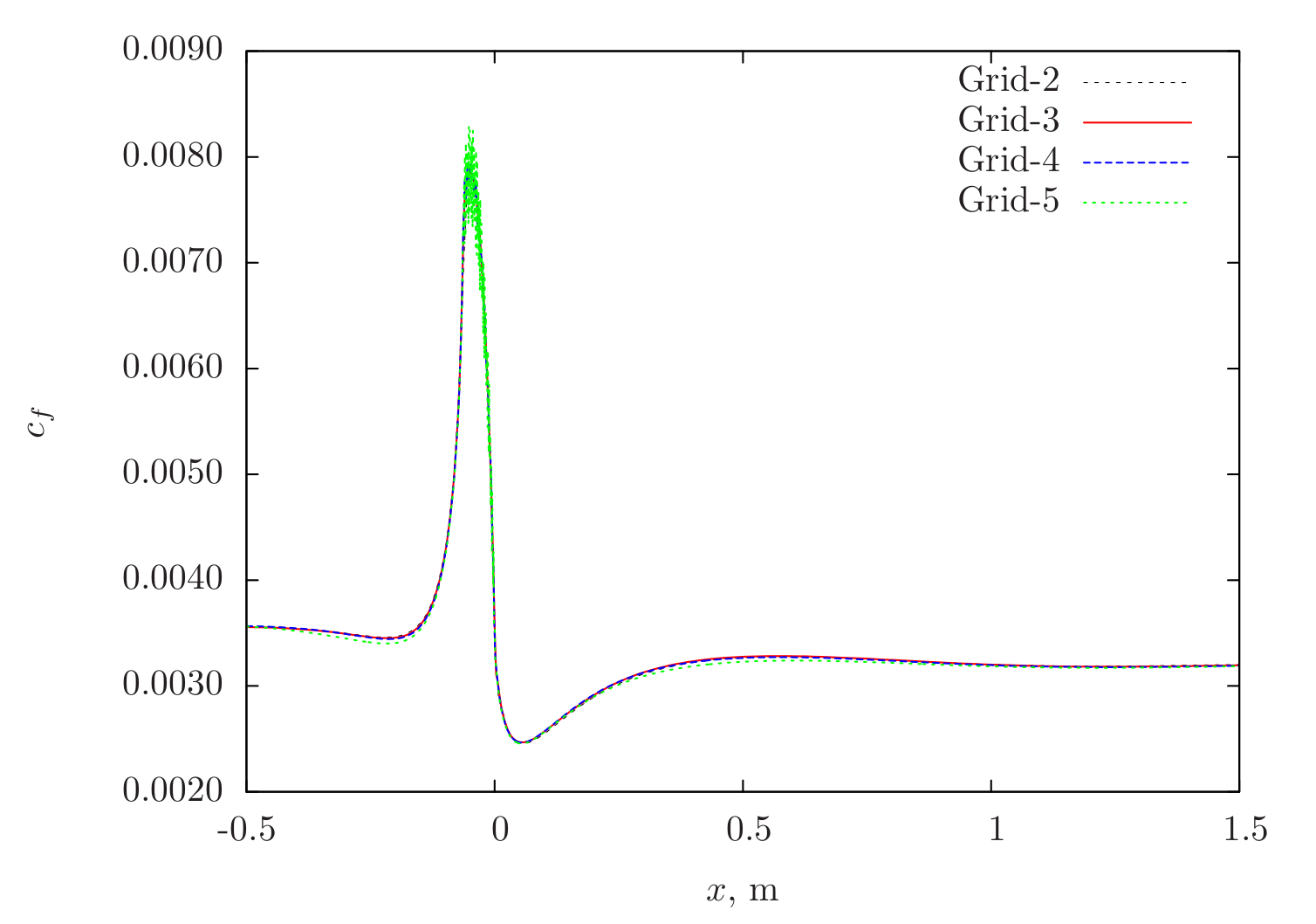
Figure 101 Skin-friction distribution obtained from Caelus simulations using SA turbulence model on the lower surface of the duct

The skin-friction coefficient comparison with CFL3D is shown in Figure 102. It should be noted that the available solution from CFL3D was for Grid-4 and hence to be consistent, Grid-4 solution from Caelus is used for comparison. In the vicinity of strong curvature region, Caelus compares very well with CFL3D, however both upstream and downstream, there seems to be some difference in the solution.

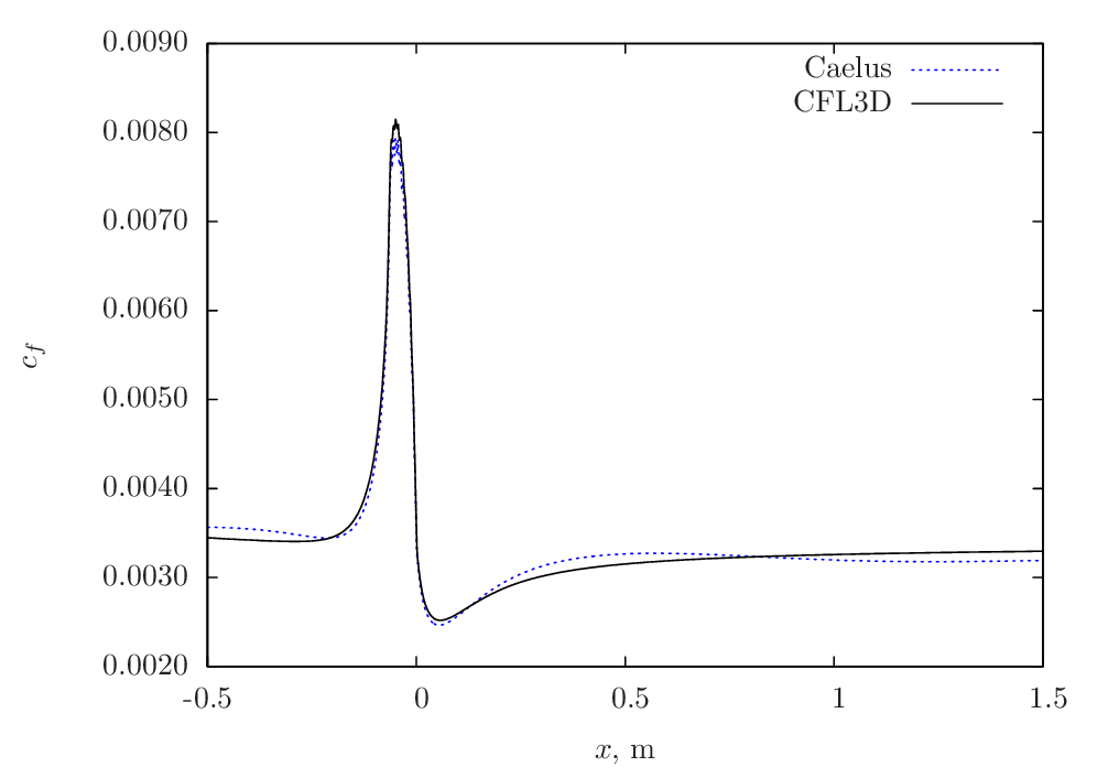
Figure 102 Skin-friction comparison between Caelus and CFL3D using SA turbulence model on the lower surface of the duct

Verification results Spalart–Allmaras Rotational/Curvature (SA-RC)

The following Figure 103 shows the grid sensitivity and verification with CFL3D data respectively. The solution that have been used for verification is obtained from Grid-4 and the trends are similar to what is noted for the SA model.

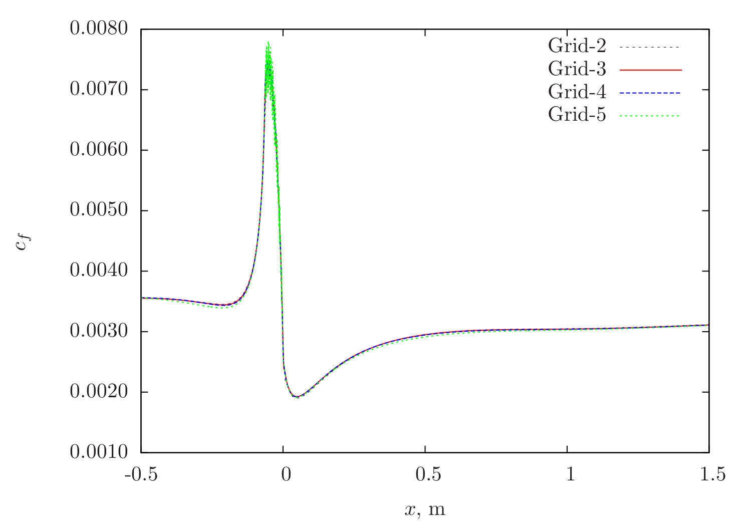
Figure 103 Skin-friction distribution obtained from Caelus simulations using SA-RC turbulence model on the lower surface of the duct

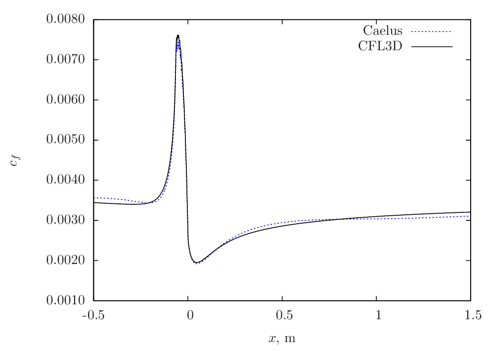
Figure 104 Skin-friction comparison between Caelus and CFL3D using SA-RC turbulence model on the lower surface of the duct

Verification results k-Omega SST

In Figure 105, the skin-friction sensitivity is shown over the lower wall obtained using Caelus with the \(k-\omega~\rm{SST}\) model. After Grid-3, not much difference in values can be noted. With Grid-5, however some oscillations can be see upstream and in the vicinity of the curvature.

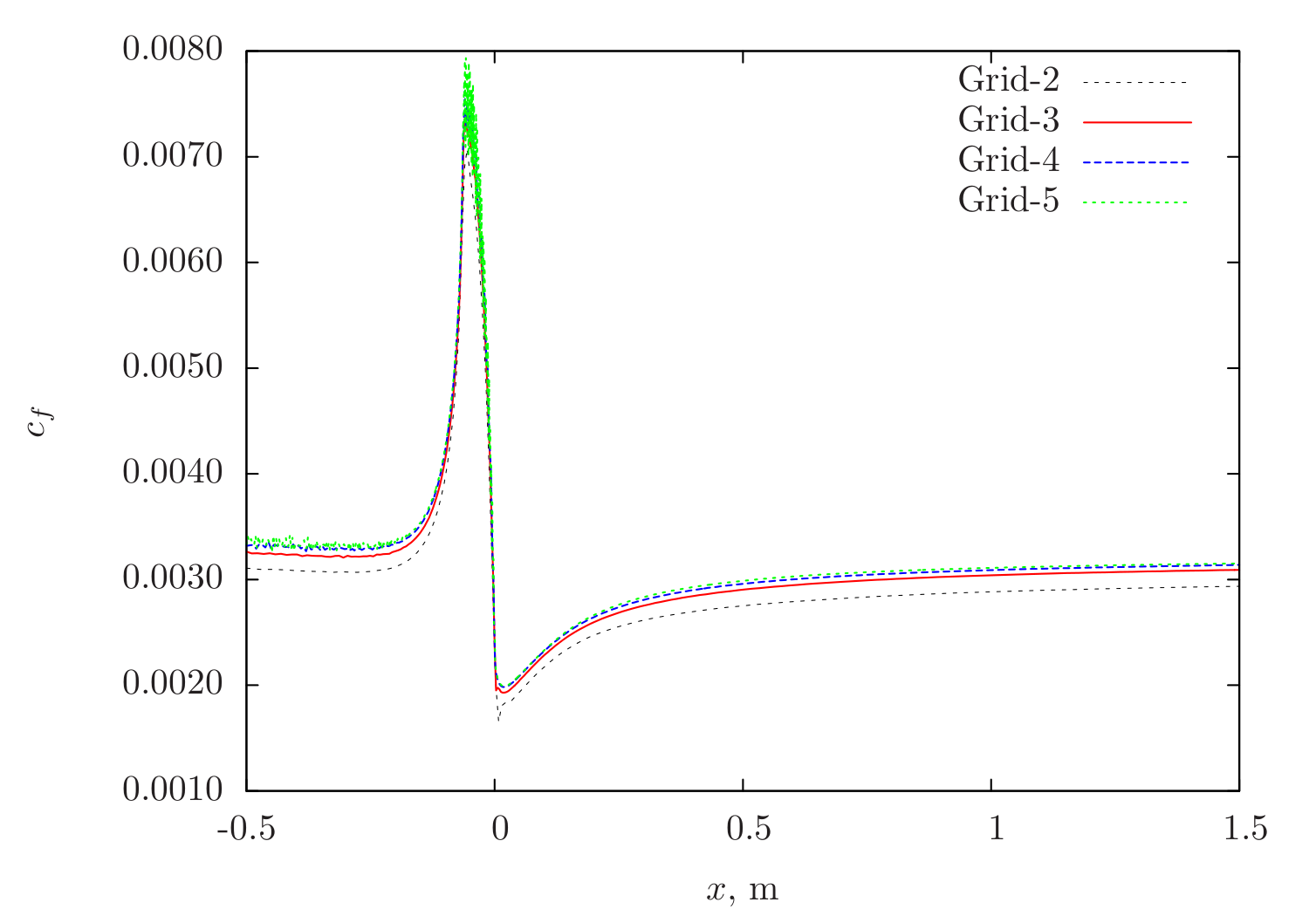
Figure 105 Skin-friction distribution obtained from Caelus simulations using \(k-\omega~\rm{SST}\) turbulence model on the lower surface of the duct

The skin-friction comparison between Caelus and CFL3D is shown in Figure 106. A very good agreement between the two is obtained.

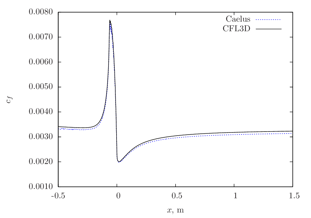
Figure 106 Skin-friction comparison between Caelus and CFL3D using \(k-\omega~\rm{SST}\) turbulence model on the lower surface of the duct

Experimental validation

This section details the experimental validation carried out for Caelus and both skin-friction and pressure coefficients obtained experimentally by Smits, A. J et al. [8] are compared. Further, CFL3D is also included. In Figure 107, skin-friction distribution obtained from Caelus using different turbulence models is compared with the experiments. Both SA-RC and \(k-\omega~\rm{SST}\) has a fair agreement with experiments down stream of the curvature, more so with the SA-RC model. However upstream they all seem to predict nearly the same values.

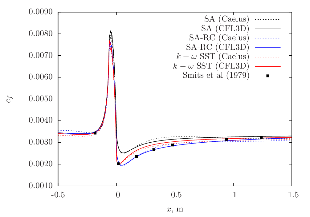
Figure 107 Skin-friction comparison between Caelus, experiments and CFL3D on the lower surface of the duct.

Figure 108 shows the comparison of pressure-coefficient (\(c_p\)) distribution with experiments and CFL3D data on the lower surface. Firstly, the solutions obtained from Caelus with the three turbulence models essentially produces the same values and matches exactly with the CFL3D data. In comparison with experiments, the agreement is very good in the upstream, vicinity of the curvature and downstream and, identical to CFL3D’s behaviour. Note that for obtaining the pressure-coefficient (\(c_p\)) values, a reference pressure (\(p_{ref}\)) is needed. However, this is not specified in Turbulence Modeling Resource for this case and hence a value of 145 Pa has been used.

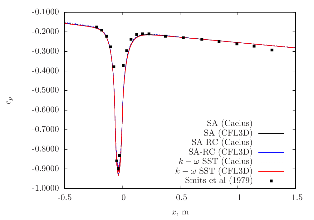
Figure 108 Pressure coefficient comparison between Caelus, experiments and CFL3D on the lower surface of the duct.

Experimental skin-friction data [8] is also available over the upper surface of the duct and is used to compare the Caelus results. Figure 109 shows the comparison. Similar to the behaviour noted for the lower surface, the SA-RC model tends to be closer to the experimental data. In general, all the three turbulence model have similar trends and agrees very closely with the CFL3D data.

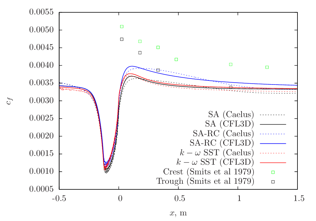
Figure 109 Skin-friction coefficient comparison between Caelus, experiments and CFL3D on the upper surface of the duct.

Conclusions

A detailed verification and validation of a turbulent flow in a convex curvature duct were carried out using Caelus 9.04 and simpleSolver. Here, three turbulence models used and the solutions were verified against CFL3D data. As a part of validation, Caelus results were compared with the experimental data obtained on both lower and upper surfaces. The comparison was good with both CFL3D as well as with experiments. This suggests that the implementation of the turbulence models is correct and is being solved accurately.

Two-dimensional Backward Facing Step

Turbulent, incompressible flow over a two-dimensional backward facing step

Nomenclature

Symbol	Definition	Units (SI)
\(a\)	Speed of sound	\(m/s\)
\(c_f\)	Skin friction coefficient	Non-dimensional
\(c_p\)	Pressure coefficient	Non-dimensional
\(H\)	Step height	\(m\)
\(I\)	Turbulent intensity	Percentage
\(k\)	Turbulent kinetic energy	\(m^2/s^2\)
\(M_\infty\)	Freestream Mach number	Non-dimensional
\(p\)	Kinematic pressure	\(Pa/\rho~(m^2/s^2)\)
\(Re_H\)	Reynolds number based on step height	Non-dimensional
\(T\)	Temperature	\(K\)
\(u\)	Local velocity in x-direction	\(m/s\)
\(u_*\)	Frictional velocity	\(m^2/s\)
\(U\)	Freestream velocity in x-direction	\(m/s\)
\(U_{ref}\)	Reference velocity	\(m/s\)
\(x\)	Distance in x-direction	\(m\)
\(z\)	Distance in z-direction	\(m\)
\(y^+\)	Wall distance	Non-dimensional
\(\epsilon\)	Turbulent dissipation	\(m^2/s^3\)
\(\mu\)	Dynamic viscosity	\(kg/m~s\)
\(\nu\)	Kinematic viscosity	\(m^2/s\)
\(\tilde{\nu}\)	Turbulence field variable	\(m^2/s\)
\(\rho\)	Density	\(kg/m^3\)
\(\tau_w\)	Wall shear stress	\(kg/m~s^2\)
\(\omega\)	Specific dissipation rate	\(1/s\)
\(\infty\)	Freestream conditions
\(t\) (subscript)	Turbulent property

Introduction

This study investigates steady turbulent, incompressible flow over a two-dimensional backward facing step at zero angle of incidence. Unlike the previous cases, the efficacy of wall functions in separated flow is evaluated for different turbulent models. The validation of these wall functions are carried out through the comparison of skin-friction coefficient (\(c_f\)) and pressure coefficient (\(c_p\)) downstream of the step with those of the experimental data. In addition to Spalart–Allmaras and \(k - \omega~\rm{SST}\), Realizable \(k-\epsilon\) turbulence model was also considered in this exercise.

Problem definition

The backward facing step configuration is obtained from the Turbulence Modeling Resource and is a widely considered case for the purpose of verification and validation. This particular study is based on the experiments carried out by Driver and Seegmiller [15]. The schematic of the step configuration in Figure 110 below as considered in the Turbulence Modeling Resource.

Figure 110 Schematic representation of the backward facing step in 2D

The height of the step (H) is chosen to be 1.0 m and is located at x = 0 m. Upstream of the step, the plate extends to 110 step heights such that a fully developed turbulent boundary layer with proper thickness exists at separation (x = 0 m). This is followed by a downstream plate which extends up to 50 step heights. The flow has a Reynolds number of 36000 based on the step height with a freestream velocity (\(U_\infty\)) in the x-direction. The inflow is assumed to be Air as a perfect gas with a temperature of 298 K, giving the value of speed of sound (\(a\)) at 346.212 m/s. A reference Mach number (\(M_\infty\)) of 0.128 is used to obtain the freestream velocity, which was \(U_\infty\) = 44.315 m/s. The kinematic viscosity was then evaluated based on the velocity and the Reynolds number. The following table summarises the freestream conditions used for the backward facing step.

Table 22 Freestream conditions

Fluid	\(Re_H\)	\(U_\infty~(m/s)\)	\(p_\infty~(m^2/s^2)\)	\(T_\infty~(K)\)	\(\nu_\infty~(m^2/s)\)
Air	\(36000\)	44.31525	\((0)\) Gauge	298.330	\(1.230979\times10^{-3}\)

As with all the previous cases, the flow is incompressible and therefore the density (\(\rho\)) does not change throughout the simulation. Further, the temperature is not accounted and has no influence on viscosity and is also held constant. However note that in Caelus, pressure and viscosity for incompressible flow are always specified as kinematic.

Turbulent Properties for Spalart–Allmaras model

The turbulent boundary conditions at the freestream used for Spalart-Allmaras model were calculated according to \(\tilde{\nu}_{\infty} = 3 \cdot \nu_\infty\) and turbulent eddy viscosity was subsequently evaluated. In the following table, the values used in the current simulation are provided:

Table 23 Turbulence freestream conditions for SA model

\(\tilde{\nu}_\infty~(m^2/s)\)	\(\nu_{t~\infty}~(m^2/s)\)
\(3.692937 \times 10^{-3}\)	\(2.590450 \times 10^{-4}\)

Turbulent Properties for k-omega SST model

The turbulent inflow boundary conditions used for \(k-\omega~\rm{SST}\) were calculated as follows and is as given in Turbulence Modeling Resource

\[k_{\infty} = \frac{3}{2} (U_\infty I)^2\]

\[\omega_{\infty} = 1 \times 10^{-6} \cdot \frac{\rho_\infty a^2_\infty}{\mu_\infty}\]

\[\nu_{t~\infty} = 0.009 \times \nu_\infty\]

The dynamic viscosity in the above equation is obtained from Sutherland formulation and the density is calculated through \(\mu/\nu\). In the table below, the turbulent properties used for the current \(k-\omega~\rm{SST}\) simulation are provided

Table 24 Turbulent freestream conditions for \(k-\omega~\rm{SST}\) Model

\(I\)	\(k_{\infty}~(m^2/s^2)\)	\(\omega_{\infty}~(1/s)\)	\(\nu_{t~~\infty}~(m^2/s)\)
\(0.061\%\)	\(1.0961 \times 10^{-3}\)	\(97.37245\)	\(1.10787 \times 10^{-5}\)

Turbulent Properties for Realizable k-epsilon model

The turbulent inflow properties used for Realizable \(k-\epsilon\) model were evaluated as follows

\[k_{\infty} = \frac{3}{2} (U_\infty I)^2\]

\[\epsilon_{\infty} = \frac{0.1643~k_{\infty}^{3/2}}{\lambda}\]

\[\nu_{t\infty} = \frac{C_\mu~k^2}{\epsilon_{\infty}}\]

where, \(\lambda\) is the turbulent length scale and is evaluated at 0.22 of the boundary layer thickness at separation (1.5H) and \(C_\mu\) is a model constant with a value 0.09. The following table provides the evaluated turbulent properties. Note that the turbulent intensity was assumed to be 1 % for this particular model.

Table 25 Turbulent freestream conditions for Realizable \(k-\epsilon\) Model

\(I\)	\(k_{\infty}~(m^2/s^2)\)	\(\epsilon_{\infty}~(m^2/s^3)\)	\(\nu_{t\infty}~(m^2/s)\)
\(1\%\)	\(294.57 \times 10^{-3}\)	\(0.079598\)	\(98.11 \times 10^{-3}\)

Computational Domain and Boundary Conditions

The computational domain simply follows the step geometry for the entire bottom region. In Figure 111 below, the boundary details in two-dimensions (\(x-z\) plane) are shown. The walls of the upstream plate, step and the downstream plate that extend between \(-110 \leq x \leq 50~m\) are modelled as no-slip wall boundary condition. Similarly, the top plate is also modelled as a no-slip wall. Upstream of the leading edge, that is, \(x \leq 110\) symmetry boundary extends for a length of 20 step heights and the inlet boundary is placed at the start of the symmetry. The outlet is placed at the end of the downstream plate, which is at \(x = 50~m\).

Figure 111 Computational domain for a 2D step (Not to scale)

Boundary Conditions and Initialisation

• Inlet

  • Velocity: Fixed uniform velocity \(u = 44.31525~m/s\) in \(x\) direction

  • Pressure: Zero gradient

  • Turbulence:

    • Spalart–Allmaras (Fixed uniform values of \(\nu_{t~\infty}\) and \(\tilde{\nu}_{\infty}\) as given in the above table)

    • \(k-\omega~\rm{SST}\) (Fixed uniform values of \(k_{\infty}\), \(\omega_{\infty}\) and \(\nu_{t~\infty}\) as given in the above table)

    • Realizable \(k-\epsilon\) (Fixed uniform value of \(k_{\infty}\), \(\epsilon_{\infty}\) and \(\nu_{t_\infty}\) as given in the above table)

• Symmetry

  • Velocity: Symmetry

  • Pressure: Symmetry

  • Turbulence: Symmetry

• No-slip wall

  • Velocity: Fixed uniform velocity \(u, v, w = 0\)

  • Pressure: Zero gradient

  • Turbulence:

    • Spalart–Allmaras:

      • \(\nu_t\): type nutUWallFunction with an initial value of \(\nu_t=0\)

      • \(\tilde{\nu}\): type fixedValue with a value of \(\tilde{\nu}=0\)

    • \(k-\omega~\rm{SST}\):

      • \(k\): type kqRWallFunction with an initial value of \(k_{\infty}\)

      • \(\omega\): type omegaWallFunction with an initial value of \(\omega_{\infty}\)

      • \(\nu_t\): type nutUWallFunction with an initial value of \(\nu_t=0\)

    • Realizable \(k-\epsilon\):

      • \(k\): type kqRWallFunction with an initial value of \(k_{\infty}\)

      • \(\epsilon\): type epsilonWallFunction with an initial value of \(\epsilon=0\)

      • \(\nu_t\): type nutUWallFunction with an initial value of \(\nu_t=0\)

• Outlet

  • Velocity: Zero gradient velocity

  • Pressure: Fixed uniform gauge pressure \(p = 0\)

  • Turbulence:

    • Spalart–Allmaras (Calculated \(\nu_{t}=0\) and Zero gradient \(\tilde{\nu}\))

    • \(k-\omega~\rm{SST}\) (Zero gradient \(k\) and \(\omega\); Calculated \(\nu_t=0\); )

    • Realizable \(k-\epsilon\) (Zero gradient \(k\) and \(\epsilon\); Calculated \(\nu_t=0\); )

• Initialisation

  • Velocity: Fixed uniform velocity \(u = 44.31525~m/s\) in \(x\) direction

  • Pressure: Zero Gauge pressure

  • Turbulence:

    • Spalart–Allmaras (Fixed uniform values of \(\nu_{t~\infty}\) and \(\tilde{\nu}_{\infty}\) as given in the above table)

    • \(k-\omega~\rm{SST}\) (Fixed uniform values of \(k_{\infty}\), \(\omega_{\infty}\) and \(\nu_{t~\infty}\) as given in the above table)

    • Realizable \(k-\epsilon\) (Fixed uniform values of \(k_{\infty}\), \(\epsilon_{\infty}\) and \(\nu_{t~\infty}\) as given in the above table)

Computational Grid

The 3D computational grid was generated using Pointwise. and was converted to Caelus format. Note that the plane of interest is in \(x-z\) directions. Further, since the flow field is assumed to be two-dimensional, the two \(x-z\) obtained as a result of a 3D grid are specified with empty boundary condition. This forces the 3D solver, simpleSolver to treat the flow in \(y\) direction as symmetry. The following figure shows the 2D grid. As noted earlier, the purpose of this exercise is to validate the wall functions and hence the grid is designed for a \(y^+ = 30\). In order to design such a gird, the first cell height (\(\Delta z\)) from wall in the wall normal (\(z\)) direction was obtained from the following set of equations

\[\Delta z = \frac{y^+~\nu}{u_*}\]

where, \(u_*\) is the frictional velocity given by

\[u_* = \sqrt{\frac{\tau_w}{\rho}}\]

In the above equation, \(\tau_w\) is the shear-stress at the wall and was be estimated using the skin-friction (\(c_f\)) relation, given as

\[\tau_w = c_f\frac{1}{2} \rho u_\infty^2\]

where, \(c_f\) was obtained for the flat-plate as given in Schlichting [7] and is shown below

\[c_f = [2~\textrm{log}(Re_x) - 0.65]^{-2.3}\]

where, \(Re_x\) is the Reynolds number based on the length of the boundary layer. In this case, it is the length developed over the upstream plate.

The 2D grid of a backward facing step in \(x-z\) is shown in Figure 112 for a \(y^+ \approx 30\). In the upstream region of the step, there are 60 cells in the streamwise and 64 in the wall normal directions respectively. Downstream of the step, there are 129 cells in the streamwise and a total of 84 cells in the normal direction. Out of 84 cells, 20 cells represent the height of the step.

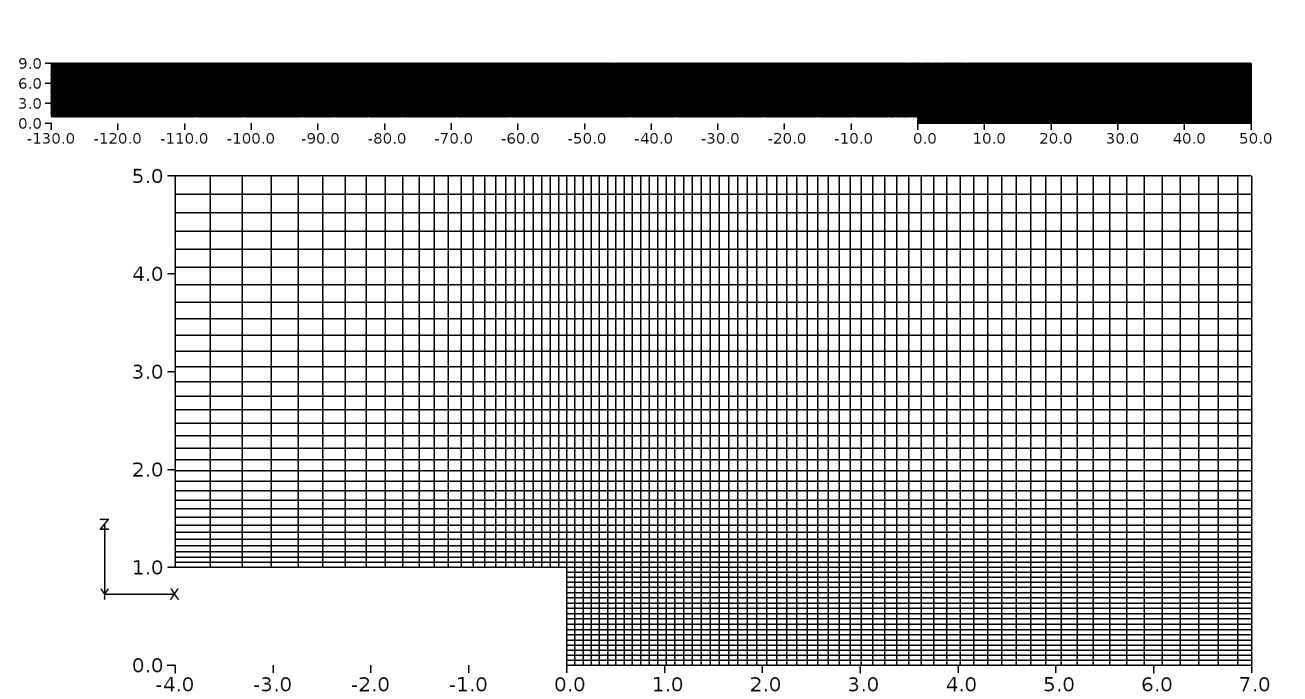
Figure 112 Backward facing step grid shown in 2D for \(y^+ \approx 30\) (Inset shows the vicinity of the step region)

Results and Discussion

The steady-state solution of turbulent flow over a two-dimensional backward facing step was obtained using Caelus 9.04. The simpleSolver was used and the simulation was run sufficiently long until the residuals for pressure, velocity and turbulent quantities were less than \(1 \times 10^{-6}\). The finite volume discretization of the gradient of pressure and velocity was carried out using linear approach. Where as the divergence of velocity and mass flux was carried out through the linear upwind method. However, for the divergence of the turbulent quantities, upwind approach was utilised. For the discretization of the Laplacian terms, again linear method was used.

Experimental validation of skin-friction coefficient

In this section, the validation carried out for Caelus based on skin-friction and pressure obtained experimentally by Driver and Seegmiller [15] is presented. The results obtained from CFL3D [1] are additionally shown and should be considered only as a reference and not as a benchmark for verification. This is because all the CFL3D results have been obtained without the use of wall functions and on a grid having \(y^+ \approx 1\). In Figure 113, skin-friction distribution obtained from Caelus using SA turbulence model is compared with the experiments. Upstream of the step, the agreement is good, however, downstream post-reattachment the skin-friction under predicts the experimental data. In both these regions of the flow, Caelus results are nearly identical to that of CFL3D suggesting that the wall-function is capturing the flow characteristics accurately. Within the separated region, there is a large discrepancy and this is due to the inherent low \(y^+\) mesh in that region, where typically a wall function becomes invalid.

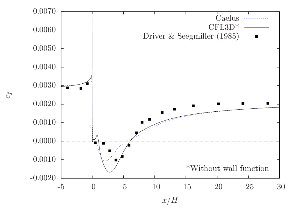
Figure 113 Skin-friction distribution obtained from Caelus simulation using SA turbulence model

Figure Figure 114 gives the comparison of skin-friction obtained from \(k-\omega~\rm{SST}\) turbulence model. The result is very similar to the one obtained from SA model. In this case, the skin-friction upstream of the step is slightly under predicted, whereas, post reattachment, it seems to be closer to experiments. In contrast with the SA result, the skin-friction is now closer to the experimental data within the separated region, particularly in the region closer to the reattachment location.

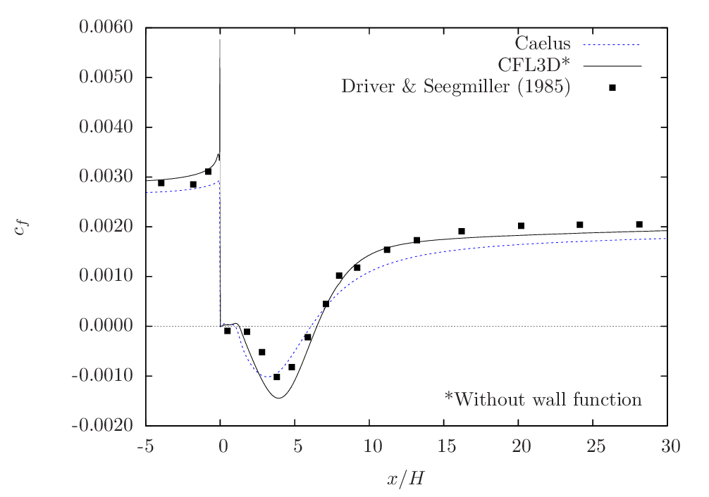
Figure 114 Skin-friction distribution obtained from Caelus simulation using \(k-\omega~\rm{SST}\) turbulence model

In Figure 115, the comparison is shown for Realizable \(k-\epsilon\) turbulence model. Note that CFL3D data was not available for this turbulence model to use as a reference. Again, similar skin-friction behaviour can be noted both upstream and downstream of the step with reasonable agreement with the experimental data. Within the separated region, there is a large difference and this could be due to the presence of low \(y^+\) mesh as discussed earlier.

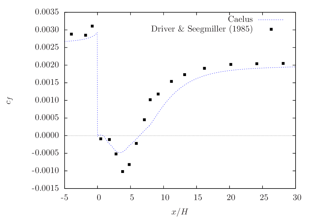
Figure 115 Skin-friction distribution obtained from Caelus simulation using Realizable \(k-\epsilon\) turbulence model

One of the key feature of modelling the backward facing step is the accurate prediction of reattachment location downstream of the step. This was determined through the location at which the reversal of skin-friction occurs over the downstream surface for each of the turbulence model considered here. In the below table, the normalised reattachment distances obtained from Caelus simulation are compared with the experimental data. Out of the three models considered here, Realizable \(k-\epsilon\) prediction is in very good agreement with the experimentally obtained value.

Table 26 Comparison of reattachment distance with the experiment data

Type	Reattachment location (\(x/H\))
Experimental	\(6.26 \pm 0.10\)
SA	\(5.55\)
\(k-\omega~\rm{SST}\)	\(6.08\)
Realizable \(k-\epsilon\)	\(6.27\)

Experimental validation of pressure coefficient

Figure 116 gives the pressure-coefficient (\(c_p\)) comparison among three Caelus simulations and the experimental data. The inclusion of CFL3D data is again only for reference and not as a benchmark comparison. All the simulations essentially produce the same trend and is consistent with the skin-friction coefficient distribution. The pressure prediction in both \(k-\omega~\rm{SST}\) and Realizable \(k-\epsilon\) are very close to each other over the entire region shown in the figure and is also in fair agreement with the experimental data. However, SA seems to show some significant deviation particularly in the region of pressure minima.

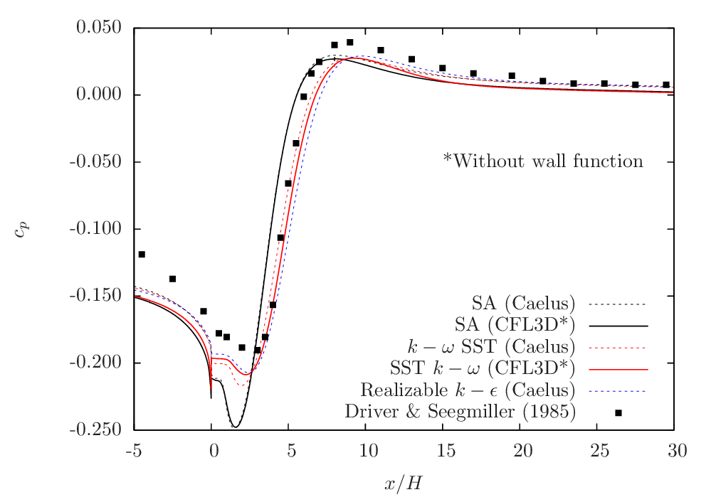
Figure 116 Pressure-coefficient comparison between Caelus and experiments over the backward facing step

Conclusions

A detailed validation of the turbulent flow over a backward facing step was carried out using Caelus 9.04 for a simpleSolver. In particular the focus was to validate wall functions for grids having \(y^+ \approx 30\). The solutions from three turbulence models were compared with both skin-friction and pressure coefficients obtained experimentally over the surface of the model. Overall, a good agreement was noted. With respect to the reattachment location, the simulated result with Realizable \(k-\epsilon\) turbulence model agreed very close to the experimental data. Considering both the skin-friction and pressure data, the implementation of the turbulence model is correct with providing accurate solutions.