Tutorials: Incompressible Laminar Flow
Laminar Flat Plate
In this tutorial, simulation of laminar incompressible flow over a two-dimensional sharp leading-edge flat plate using Caelus 9.04 is introduced here. First, pre-requisites to begin a Caelus simulation is discussed followed by various dictionary entries defining fluid properties, boundary conditions, solver setting, etc that are needed. Finally, the presence of laminar boundary layer is visualised using velocity contours. Here, the basic procedures of running Caelus is shown in sufficient detail such that the user feels comfortable with the usage.
Objectives
With the completion of this tutorial, the user will be familiar with setting up Caelus simulation for steady, laminar, incompressible flow over flat-plates in two-dimensions and subsequently post-processing the results. Following are some of the steps carried out in this tutorial
- Background
A brief description about the problem
Geometry and freestream details
- Grid generation
Computational domain and boundary details
Computational grid generation
Exporting grid to Caelus
- Problem definition
Directory structure
Setting up boundary conditions, physical properties and control/solver attributes
- Execution of the solver
Monitoring the convergence
Writing the log files
- Results
Visualisation of the laminar boundary layer
Pre-requisites
It is assumed that the user is familiar with the Linux command line environment using a terminal or Caelus-console (for Windows OS) and that Caelus is installed correctly with appropriate environment variables set. The grid used here is generated using Pointwise and the user is free to use their choice of grid generation tool having exporting capabilities to the Caelus grid format.
Background
The flow over a flat-plate presents an ideal case where initial steps of a Caelus simulation can be introduced to the user in easy steps. Here, laminar, incompressible flow over a sharp-leading edge plate is solved in a time-accurate approach. This results in the formation of laminar boundary layer which is then compared with the famous Blasius [6] analytical solution in the form of a non-dimensional shear stress distribution (skin-friction coefficient). For more details, the user is suggested to refer the validation of flat-plate in section Flat plate validation.
The length of the flat-plate considered here is \(L = 0.3048~m\) with a Reynolds number based on the total length of \(Re = 200,000\). A schematic of the geometry is shown in Figure 1, wherein \(U\) is the flow velocity in \(x\) direction. An inflow temperature of \(T = 300~K\) can assumed for the fluid air which corresponds to a kinematic viscosity (\(\nu\)) of \(\nu = 1.5896306 \times 10^{-5}~m^2/s\). Using the values of \(Re\), \(L\) and \(\nu\), we can evaluate the freestream velocity to \(U = 10.4306~m/s\).

Figure 1 Schematic of the flat-plate flow
In the following table, details of the freestream conditions are provided.
Fluid |
\(L~(m)\) |
\(Re\) |
\(U~(m/s)\) |
\(p~(m^2/s^2)\) |
\(T~(K)\) |
\(\nu~(m^2/s)\) |
|---|---|---|---|---|---|---|
Air |
0.3048 |
200,000 |
69.436113 |
Gauge (0) |
300 |
\(1.58963\times10^{-5}\) |
Grid Generation
As noted earlier, Pointwise has been used here to generate a hexahedral grid. Specific details pertaining to its usage are not discussed here, rather a more generic discussion is given about the computational domain and boundary conditions. This would facilitate the user to obtain a Caelus compatible grid using their choice of grid generating tool.
The computational domain is a rectangular block encompassing the flat-plate. The below (Figure 2) shows the details of the boundaries that will be used in two-dimensions (\(x-y\) plane). First, the flat-plate, which is our region of interest (highlighted in blue) is extended between \(0\leq x \leq 0.3048~m\). Because of viscous nature of the flow, the velocity at the wall is zero which can be represented through a no-slip boundary (\(u, v, w = 0\)). Upstream of the leading edge, a slip boundary will be used to simulate a freestream flow approaching the flat-plate. However, downstream of the plate, it would be ideal to further extend up to three plate lengths (highlighted in green) with no-slip wall. This would then ensure that the boundary layer in the vicinity of the trailing edge is not influenced by outlet boundary. Since the flow is incompressible (subsonic), the disturbance caused by the pressure can propagate both upstream as well as downstream. Therefore, the placement of the inlet and outlet boundaries are to be chosen to have minimal or no effect on the solution. The inlet boundary as shown will be placed at start of the slip-wall at \(x = -0.06~m\) and the outlet at the exit plane of the no-slip wall (green region) at \(x = 1.2192~m\). Both inlet and outlet boundary are between \(0\leq y \leq 0.15~m\). A slip-wall condition is used for the entire top boundary.

Figure 2 Flat-plate computational domain
The 2D structured grid is shown in Figure 3. Since Caelus is a 3D solver, it necessitates the grid to be in 3D. Therefore, the 3D grid should be obtained through extruding the 2D gird in the \(z\) direction by a minimum of one-cell thick. The final 3D grid should be then exported to Caelus format (polyMesh). The two \(x-y\) planes obtained as a result of grid extrusion need boundary conditions to be specified. As the flow over a flat-plate is generally 2D, we do not need to solve the flow in the third dimension. This can easily be achieved in Caelus by specifying empty boundary condition for each of those two planes.
Note
A velocity value of \(w=0\) needs to be specified at appropriate boundaries although no flow is solved in the \(z\) direction.
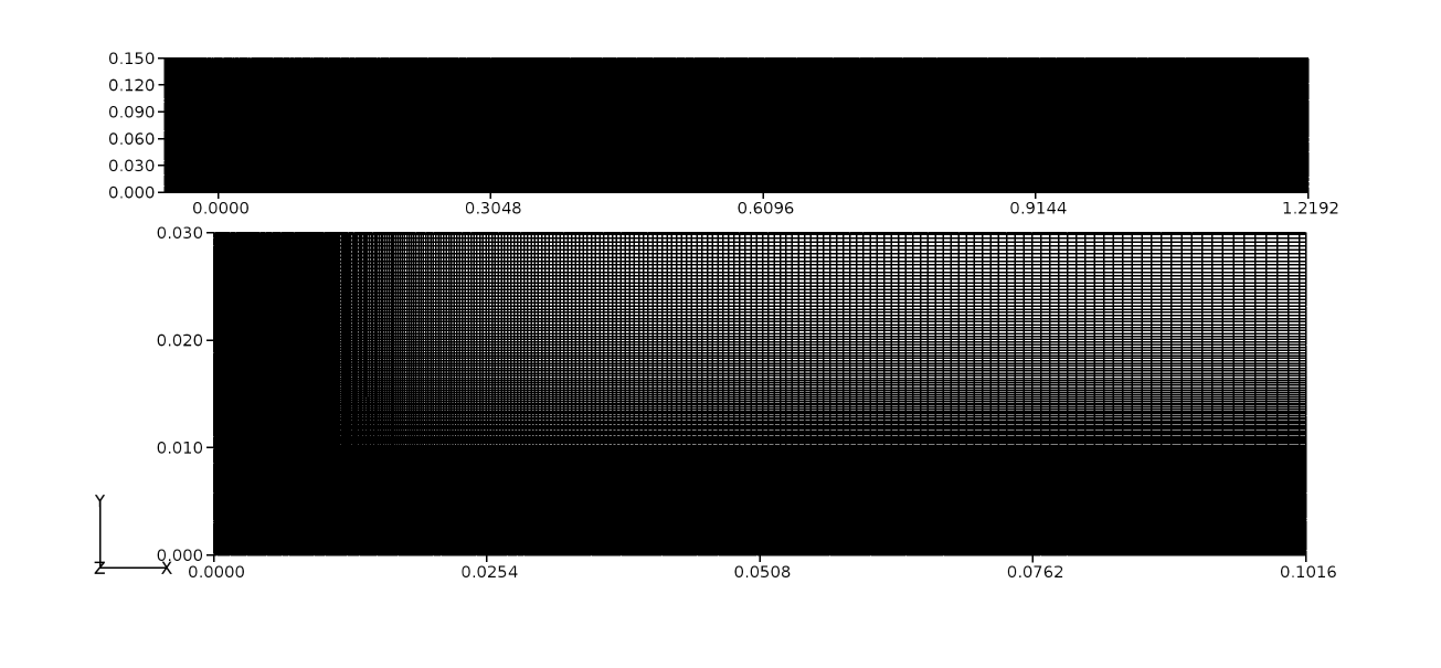
Figure 3 Flat-plate computational grid
The flat-plate has a total of 400 cells over the region of interest between \(0 \leq x \leq 0.3048~m\) and 286 cells in the no-slip wall that extends for an additional 3 plate lengths (green region in the above figure). In the wall normal direction, 298 cells are used and sufficient refinement close to the wall was made to ensure that accurate boundary layer is captured.
Problem definition
Several important instructions would be shown here to set-up the flat-plate problem along with the detail of configuration files used. A full working case can be found in:
/tutorials/incompressible/simpleSolver/laminar/ACCM_flatPlate2D
However,the user is free to start the case setup from scratch consistent with the directory stucture discussed below.
Directory Structure
Note
All commands shown here are entered in a terminal window, unless otherwise mentioned
In order to set-up the problem, three main sub-directories containing all the relevant information are used. Caelus requires time, constant and system sub-directories. Since we begin the simulation at time \(t = 0~s\), the time sub-directory should be just 0.
The 0 sub-directory is where additional two files, p and U for pressure (\(p\)) and velocity (\(U\)) respectively are kept. The contents of these two files sets the dimensions, initialisation and boundary conditions to the problem, which also form three principle entries required.
It should be noted that Caelus is case sensitive and therefore the user should set-up the directories (if applicable), files and the contents identical to what is mentioned here.
Boundary Conditions and Solver Attributes
Boundary Conditions
First let us look at setting up the boundary conditions. Referring back to Figure 2, following are the boundary conditions that need to be specified:
- Inlet
Velocity: Fixed uniform velocity \(u = 10.4306~m/s\) in \(x\) direction
Pressure: Zero gradient
- Slip wall
Velocity: slip
Pressure: slip
- No-slip wall
Velocity: Fixed uniform velocity \(u, v, w = 0\)
Pressure: Zero gradient
- Outlet
Velocity: Zero gradient velocity
Pressure: Fixed uniform gauge pressure \(p = 0\)
- Initialisation
Velocity: Fixed uniform velocity \(u = 10.4306~m/s\) in \(x\) direction
Pressure: Zero Gauge pressure
Now let us look at the contents and significance of each file in these sub-directories beginning with the pressure (\(p\)) file.
/*---------------------------------------------------------------------------*\
Caelus 9.04
 Web:      www.caelus-cml.com
\*---------------------------------------------------------------------------*/
FoamFile
{
    version     2.0;
    format      ascii;
    class       volScalarField;
    location    "0";
    object      p;
}
// * * * * * * * * * * * * * * * * * * * * * * * * * * * * * * * * * * * * * //

dimensions      	[0 2 -2 0 0 0 0];

internalField   	uniform 0;

boundaryField
{
    downstream
    {
        type            zeroGradient;
    }
    inflow
    {
        type            zeroGradient;
    }
    outflow
    {
        type            fixedValue;
        value           uniform 0;
    }
    symm-left
    {
        type            empty;
    }
    symm-right
    {
        type            empty;
    }
    top
    {
        type            slip;
    }
    upstream
    {
        type            slip;
    }
    wall
    {
        type            zeroGradient;
    }
}


// ************************************************************************* //
The above file begins with a dictionary named FoamFile which contains standard set of keywords for version, format, location, class and object names. The following are the principle entries required for this case.
dimensionis used to specify the physical dimensions of the pressure field. Here, pressure is defined in terms of kinematic pressure with the units (\(m^2/s^2\)) written as
[0 2 -2 0 0 0 0]
internalFieldis used to specify the initial conditions. It can be either uniform or non-uniform. Since we have a 0 initial uniform gauge pressure, the entry is
uniform 0
boundaryFieldis used to specify the boundary conditions. In this case its the boundary conditions for pressure at all the boundary patches.
Similarly, the file U, shown below sets the boundary conditions for velocity.
/*---------------------------------------------------------------------------*\
Caelus 9.04
 Web:      www.caelus-cml.com
\*---------------------------------------------------------------------------*/
FoamFile
{
    version     2.0;
    format      ascii;
    class       volVectorField;
    location    "0";
    object      U;
}
// * * * * * * * * * * * * * * * * * * * * * * * * * * * * * * * * * * * * * //

dimensions      	[0 1 -1 0 0 0 0];

internalField   	uniform (10.4306 0 0);

boundaryField
{
    downstream
    {
        type            fixedValue;
        value           uniform (0 0 0);
    }
    inflow
    {
        type            fixedValue;
        value           uniform (10.4306 0 0);
    }
    outflow
    {
        type            zeroGradient;
    }
    symm-left
    {
        type            empty;
    }
    symm-right
    {
        type            empty;
    }
    top
    {
        type            slip;
    }
    upstream
    {
        type            slip;
    }
    wall
    {
        type            fixedValue;
        value           uniform (0 0 0);
    }
}


// ************************************************************************* //
The principle entries for velocity field are self explanatory and the dimension are typical for velocity with units \(m/s\) ([0 1 -1 0 0 0 0]). Since we initialise the flow with a uniform freestream velocity, we set the internalField to uniform (10.43064759 0 0) representing three components of velocity. In a similar manner, inflow, wall and downstream boundary patches have three velocity components.
At this stage it is important to ensure that the boundary conditions (inflow, outflow, top, etc) specified in the above files should be the grid boundary patches (surfaces) generated by the grid generation tool and their names are identical. Further, the two boundaries in \(x-y\) plane obtained due to grid extrusion have been named as symm-left and symm-right with specifying empty boundary conditions forcing Caelus to assume the flow to be in two-dimensions. This completes the setting up of boundary conditions.
Grid file and Physical Properties
The flat-plate grid files that is generated in the Caelus format resides in the constant/polyMesh sub-directory. It contains information relating to the points, faces, cells, neighbours and owners of the mesh.
In addition, the physical properties are specified in various different files present in the directory constant. In the transportProperties file, transport model and kinematic viscosity are specified. The contents of this file are as follows
/*------------------------------------------------------------------------------*
Caelus 9.04
Web:   www.caelus-cml.com
\*------------------------------------------------------------------------------*/

FoamFile
{
	version				2.0;
	format				ascii;
	class				dictionary;
	location			"constant";
	object				transportProperties;
}

//--------------------------------------------------------------------------------

transportModel				Newtonian;

nu					nu [0 2 -1 0 0 0 0] 1.5896306e-5;
As the flow is Newtonian, the transportModel is specified with Newtonian keyword and the value of kinematic viscosity (nu) is given which has the units \(m^2/s\) ([0 2 -1 0 0 0 0]).
The next file is the turbulenceProperties file, where the type of simulation is specified.
/*------------------------------------------------------------------------------*
Caelus 9.04
Web:   www.caelus-cml.com
\*------------------------------------------------------------------------------*/

FoamFile
{

	version				2.0;
	format				ascii;
	class				dictionary;
	location			"constant";
	object				turbulenceProperties;
}

//--------------------------------------------------------------------------------

simulationType				laminar;
Since the flow here is laminar, the simulationType would be laminar. Similarly, in the RASProperties file, RASModel is set to laminar as shown below.
/*-------------------------------------------------------------------------------*
Caelus 9.04
Web:   www.caelus-cml.com
\*------------------------------------------------------------------------------*/

FoamFile
{
	version				2.0;
	format				ascii;
	class				dictionary;
	location			"constant";
	object				RASProperties;
}

//--------------------------------------------------------------------------------

RASModel				laminar;


turbulence				off;

printCoeffs				on;
Controls and Solver Attributes
The files required to control the simulation and specifying the type of discretization method along with the linear solver settings are present in the system directory.
The controlDict file is shown below:
/*------------------------------------------------------------------------------*
Caelus 9.04
Web:   www.caelus-cml.com
\*------------------------------------------------------------------------------*/

FoamFile
{
	version				2.0;
	format				ascii;
	class				dictionary;
	location			"system";
	object				controlDict;
}

//-------------------------------------------------------------------------------

application				simpleSolver;

startFrom				startTime;

startTime				0;

stopAt					endTime;

endTime					2000;

deltaT					1;

writeControl				runTime;

writeInterval				500;

purgeWrite				0;

writeFormat				ascii;

writePrecision				6;

writeCompression 			uncompressed;

timeFormat				general;

timePrecision				6;

runTimeModifiable			true;
Here, the application simpleSolver refers to the SIMPLE solver that will be used. We also begin the simulation at \(t = 0~s\), which logically explains the need for 0 directory where the data files are read at the beginning of the run. Therefore, we need to set the keyword startFrom to startTime, where startTime would be 0. Since simpleSolver is a steady-state solver, the keyword endTime corresponds to the total number of iterations.The interval at which output files are written is controlled by writeControl and writeInterval keywords.
The discretization schemes and parameters are specified through the fvSchemes file, shown below
/*------------------------------------------------------------------------------*
Caelus 9.04
Web:   www.caelus-cml.com
\*------------------------------------------------------------------------------*/

FoamFile
{
	version				2.0;
	format				ascii;
	class				dictionary;
	object				fvSchemes;
}

//------------------------------------------------------------------------------

ddtSchemes
{
	default				steadyState;
}

gradSchemes
{
	default				Gauss	linear;
	grad(p)				Gauss	linear;
	grad(U)				Gauss	linear;
}

divSchemes
{
	default				none;
	div(phi,U)			Gauss	linearUpwind	grad(U);
	div((nuEff*dev(T(grad(U)))))	Gauss 	linear;
}

laplacianSchemes
{
	default					none;
	laplacian(nu,U)			Gauss	linear	corrected;
	laplacian(nuEff,U)		Gauss	linear	corrected;
	laplacian(p)			Gauss	linear	corrected;
	laplacian(rAUf,p)		Gauss 	linear	corrected;
	laplacian((1|A(U)),p) 		Gauss 	linear 	corrected;
}

interpolationSchemes
{
	default				linear;
	interpolate(HbyA)		linear;
}

snGradschemes
{
	default				corrected;
}
Here, the discretization schemes for finite volume discretization of time-derivative, gradient, divergence and Laplacian terms are specified.
The linear solver controls and tolerances are set in fvSolution as given below
/*-------------------------------------------------------------------------------*
Caelus 9.04
Web:   www.caelus-cml.com
\*------------------------------------------------------------------------------*/
FoamFile
{
        version                         2.0;
        format                          ascii;
        class                           dictionary;
        location                        "system";
        object                          fvSolution;
}

//------------------------------------------------------------------------------

solvers
{
        p
        {
            solver          PCG;
            preconditioner
            {
                	preconditioner  		GAMG;
                	smoother        		SSGS;
	                cacheAgglomeration 		true;
        	        nCellsInCoarsestLevel 		10;
                	agglomerator    		algebraicPair;
                	mergeLevels     		1;
            }
            tolerance       1e-08;
            relTol          0.01;
            maxIter         500;
        }
        U
        {
                solver                  PBiCGStab;
                preconditioner          USGS;
                tolerance               1e-7;
                relTol                  0.1;
        }

}

SIMPLE
{
        nNonOrthogonalCorrectors        0;
        pRefCell                        0;
        pRefValue                       0;
        consistent  true;
}

// relexation factors

relaxationFactors
{
        p                               1.0;
        U                               0.7;
}
Different linear solvers are used here to solve pressure and velocity. The GAMG preconditioner is applied to improve convergence of the p solver. Also, by setting the keyword consistent to true, SIMPLEC solver is used and therefore a relaxation factor of 1.0 is applied for p.
The set-up of the directory structure along with the relevant files are completed. Let us verify again by typing the following command (on Linux and Caelus-console prompt) and the directory tree should be identical to the one shown below
tree
.
├── 0
│   ├── p
│   └── U
├── constant
│   ├── polyMesh
│   │   ├── boundary
│   │   ├── faces
│   │   ├── neighbour
│   │   ├── owner
│   │   └── points
│   ├── RASProperties
│   ├── transportProperties
│   └── turbulenceProperties
└── system
    ├── controlDict
    ├── fvSchemes
    └── fvSolution
Execution of the solver
Before execution of the solver, renumbering of the grid or mesh needs to be performed as well as checking the quality of the grid. Renumbering the grid-cell list is vital to reduce the matrix bandwidth while the quality check gives us the mesh statistics. Renumbering and mesh quality can be determined by executing the following from the top directory
caelus run -- renumberMesh -overwrite
caelus run -- checkMesh
It is suggested for the user to take note of the bandwidth before and after the mesh renumbering. When the checkMesh is performed, the following information is given as an output
/*---------------------------------------------------------------------------*\
 Caelus 8.04
 Web:      www.caelus-cml.com
\*---------------------------------------------------------------------------*/
// * * * * * * * * * * * * * * * * * * * * * * * * * * * * * * * * * * * * * //

Checking geometry...
    Overall domain bounding box (-0.06 0 0.03) (1.2192 0.15 0.055)
    Mesh (non-empty, non-wedge) directions (1 1 0)
    Mesh (non-empty) directions (1 1 0)
    All edges aligned with or perpendicular to non-empty directions.
    Boundary openness (5.80542e-19 1.1194e-17 1.1403e-14) OK.
    Max cell openness = 2.2093e-16 OK.
    Max aspect ratio = 55.555 OK.
    Minimum face area = 1e-08. Maximum face area = 0.000138887.  Face area magnitudes OK.
    Min volume = 2.5e-10. Max volume = 2.50831e-07.  Total volume = 0.004797.  Cell volumes OK.
    Mesh non-orthogonality Max: 0 average: 0
    Non-orthogonality check OK.
    Face pyramids OK.
    Mesh skewness Max: 3.85044e-13 average: 9.40402e-15 OK.
    Coupled point location match (average 0) OK.

Mesh OK.

End
The mesh non-orthogonality as reported above is 0 and therefore no non-orthogonal corrections are needed in this case. In the case of mesh non-orthogonality being high, certain number of corrections are to be accounted for which can be set in the fvSolution file with the keyword nNonOrthogonalCorrectors. The next step is to execute the solver and monitoring the progress of the solution. The solver is always executed from the top directory which is ACCM_flatPlate2D in our case as below
caelus run -l my-flat-plate.log -- simpleSolver
Now the simulation begins and the output of the solution process is written to the log file, my-flat-plate.log. In another the terminal window the solver process a ca nbe watched through plotting of the residuals
caelus logs -w my-flat-plate.log
Now the convergence of pressure can be seen with respect to number of iterations along with other convergence properties.
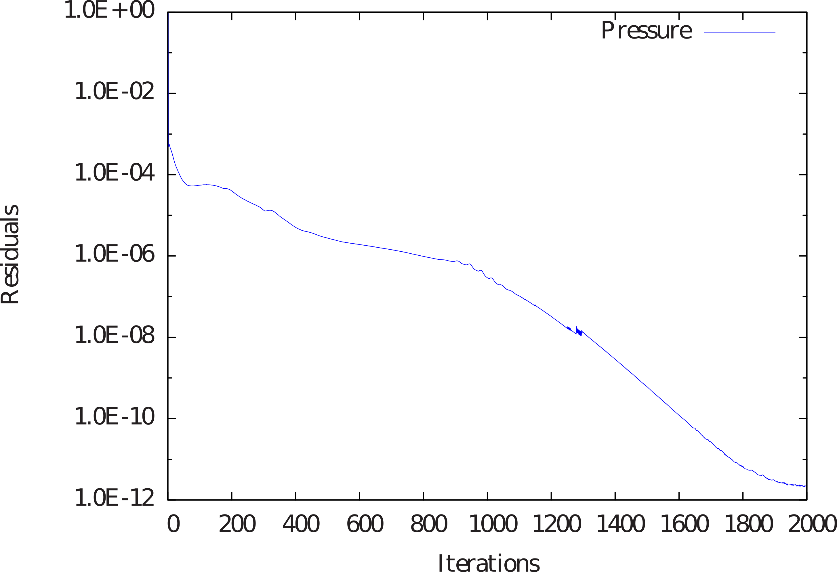
Figure 4 Convergence of pressure with respect to number of iterations.
Results
A brief qualitative data of the simulated flat-plate results are given here. Since the aim here is to obtained the steady solution, the results therefore represent the final steady state condition. In Figure 5, the contours of velocity magnitude are shown which highlights the development of the boundary layer. Since the Reynolds number of the flow is high, thickness of the boundary layer is quite thin in comparison to the length of the plate.
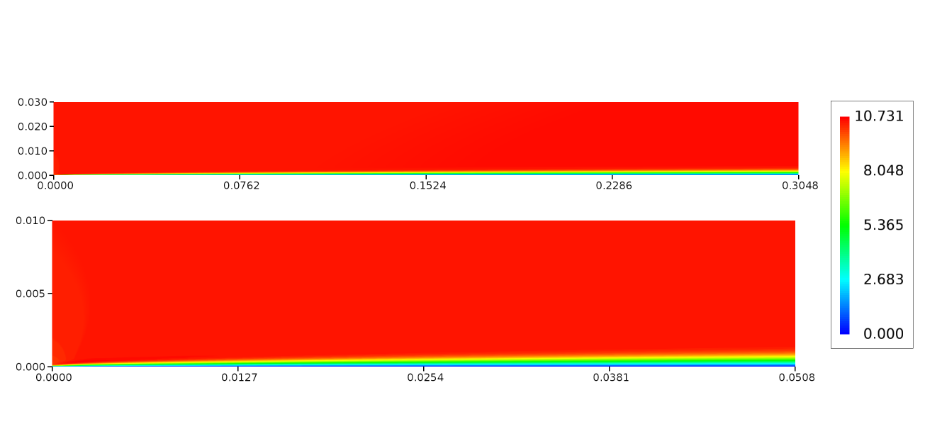
Figure 5 Contour of velocity magnitude over the flat-plate
Tee Junction
This tutorial introduces the steady, laminar flow through a two-dimensional \(90^\circ\) tee-junction. Here, we will be using Caelus 9.04 and some of the basic requirements to begin a Caelus simulation will be shown. These include, specifying input data defining boundary conditions, fluid properties and discretization/solver settings. At the end, visualisation is carried out to look at the pressure and velocity contours within the tee-junction. The details in running a Caelus simulation for the tee-junction will be shown in sufficient detail so that the user is able to repeat the numerical experiment.
Objectives
Through the completion of this tutorial, the user will be able to set-up the Caelus simulation for laminar, incompressible flow through a two-dimensional junction and subsequently estimate the flow-split. Following are the steps that will be carried out in this tutorial
- Background
A brief description about the problem
Geometry and flow conditions
- Grid generation
Computational domain and boundary details
Computational grid generation
Exporting grid to Caelus
- Problem definition
Directory structure
Setting up boundary conditions, physical properties and control/solver attributes
- Execution of the solver
Monitoring the convergence
Writing the log files
- Results
Visualising the flow inside the tee-junction
Pre-requisites
It is assumed that the user is familiar with the Linux command line environment using a terminal or Caelus-console (for Windows OS) and that Caelus is installed correctly with appropriate environment variables set. The grid used here is generated using Pointwise and the user is free to use their choice of grid generation tool having exporting capabilities to the Caelus grid format.
Background
The flow in a tee-junction presents with a simple introduction in carrying out separated flow simulation in Caelus. Because of the presence of a side branch, the flow separates forming a recirculating region. This in turn affects the mass flow through main and side branches altering the flow splits. For more details, the user can refer to the validation example show in Tee Junction.
A schematic of the tee-junction geometry is shown in Figure 6. Here, \(L = 3.0~m\) and \(W = 1.0~m\) with a Reynolds number of \(Re_w = 300\) based on the side branch width. The velocity (\(V\)) is assumed to be \(1~m/s\) in the \(y\) direction for simplicity. With these flow parameters, the kinematic viscosity can be evaluated to \(\nu = 0.00333~m^2/s\).

Figure 6 Tee-junction geometry
In the table, the flow parameters are provided.
\(Re\) |
\(V~(m/s)\) |
\(p~(m^2/s^2)\) |
\(\nu~(m^2/s)\) |
|---|---|---|---|
300 |
1.0 |
0 Gauge |
0.00333 |
Grid Generation
A hexahedral grid is generated for the tee-junction grid using Pointwise. Specific grid generation details are not discussed here, however information regarding the computational domain and boundary conditions are provided. With this, the user will be able to generate an equivalent grid using their choice of tool.
The computational domain should follow the tee-junction geometry and the details are shown in Figure 7. Due to viscous nature of the flow, the velocity at the walls is zero, which should be represented through a no-slip boundary condition (\(u, v, w = 0\)) highlighted in blue. A fully developed laminar flow with a parabolic velocity profile will also be applied as a profile boundary at the inlet. This would ensure that the velocity is fully developed before it approaches the side branch, otherwise requiring to have sufficient length in main branch for the flow to develop. As shown in the geometry, the domain will have two outlets, one at the end of the main channel and the other at the end of side branch. Also of further importance is that the exit pressures at the two outlets are set equal.

Figure 7 Tee junction Computational Domain
The 2D structured grid is shown in Figure 8 for a \(x-y\) plane. Caelus is a 3D solver and hence requires a 3D grid although the flow here is assumed to be two-dimensional. The 3D grid was obtained by extruding the 2D grid in the third (\(z\) - direction) dimension by one-cell thick. The two \(x-y\) planes obtained as a result of mesh extrusion needs boundary conditions to be specified. As the flow is assumed to be 2D, we do not need to solve the flow in \(z\) direction and this was achieved by specifying empty boundary condition for each of those two planes.
Note
A velocity value of \(w=0\) needs to be specified at appropriate boundaries although no flow is solved in the \(z\) direction.

Figure 8 Tee junction Structured Grid
A coarse grid with a total of 2025 cells is made for the tee-junction of which, 90 cells are distributed along the height of the main channel, and 45 along the length of the side branch. The distribution is such that a dimensional length, \(L = 1~m\) has a total of 45 cells and this gives a distribution of \((2/3)45 = 30\) cells for the \((2/3) L\) segment of the main channel. The width \(W\) consists of 15 cells.
Problem definition
We begin with instructions to set-up the tee-junction problem and subsequently configuring the required input files. A full working case can be found in the following location
/tutorials/incompressible/simpleSolver/laminar/ACCM_teeJunction
However,the user is free to start the case setup from scratch consistent with the directory stucture discussed below.
Directory Structure
Note
All commands shown here are entered in a terminal window, unless otherwise mentioned
For setting up the problem the following directories are needed:time, constant and system, where relevant files are placed. In this case, the time directory would be named 0 as we begin the simulation at time \(t = 0~s\).
In the 0 sub-directory, two additional files p and U for pressure (\(p\)) and velocity (\(U\)) are present. The input contents of these two files set the dimensions, initial and boundary conditions to the problem. These three forms the principle entries required.
It should be noted that Caelus is case sensitive and therefore the user should set-up the directories (if applicable), files and the contents identical to what is mentioned here.
Boundary Conditions and Solver Attributes
Boundary Conditions
Referring to Figure 7, the following boundary conditions will be applied:
- Inlet
Velocity: Parabolic velocity profile; average velocity of \(v = 1.0~m/s\) in \(y\) direction
Pressure: Zero gradient
- No-slip wall
Velocity: Fixed uniform velocity \(u, v, w = 0\)
Pressure: Zero gradient
- Outlet-1
Velocity: Zero gradient velocity
Pressure: Fixed uniform gauge pressure \(p = 0\)
- Outlet-2
Velocity: Zero gradient velocity
Pressure: Fixed uniform gauge pressure \(p = 0\)
- Initialisation
Velocity: Fixed uniform velocity \(u, v, w = 0\)
Pressure: Zero Gauge pressure
The first quantity to define would be the pressure (\(p\)) and this is done by in file p, which can be opened using a text editor.
/*------------------------------------------------------------------------------*
Caelus 9.04
Web:   www.caelus-cml.com
\*-----------------------------------------------------------------------------*/
FoamFile
{
	version				2.0;
	format				ascii;
	class				volScalarField;
	location			"0";
	object				p;
}

//-------------------------------------------------------------------------------

dimensions				[0 2 -2 0 0 0 0];

internalField				uniform 0;

boundaryField
{
	wall
	{
		type			zeroGradient;
	}
	inlet
	{
		type			zeroGradient;
	}
	outlet-1
	{
		type			fixedValue;
		value			uniform	0;
	}
	outlet-2
	{
		type			fixedValue;
		value			uniform 0;
	}
	symm-left-right
	{
		type			empty;
	}
}
As we can see, the above file begins with a dictionary named FoamFile which contains standard set of keywords such as version, format, location, class and object names. This is followed by the principle elements
dimensionis used to specify the physical dimensions of the pressure field. Here, pressure is defined in terms of kinematic pressure with the units (\(m^2/s^2\)) written as
[0 2 -2 0 0 0 0]
internalFieldis used to specify the initial conditions. It can be either uniform or non-uniform. Since we have a 0 initial uniform gauge pressure, the entry is
uniform 0;
boundaryFieldis used to specify the boundary conditions. In this case its the boundary conditions for pressure at all the boundary patches.
In a similar manner, the input data for the velocity file is shown below
/*------------------------------------------------------------------------------*
Caelus 9.04
Web:   www.caelus-cml.com
\*-----------------------------------------------------------------------------*/
FoamFile
{
	version				2.0;
	format				ascii;
	class				volVectorField;
	object				U;
}

//-------------------------------------------------------------------------------

dimensions				[0 1 -1 0 0 0 0];

internalField				uniform (0 0 0);

boundaryField
{
	wall
	{
		type			fixedValue;
		value			uniform (0 0 0);
	}
	inlet
   	{
		type			groovyBC;
		variables		"Vmax=1.0;xp=pts().x;minX=min(xp);maxX=max(xp);para=-(maxX-pos().x)*(pos().x-minX)/(0.25*pow(maxX-minX,2))*normal();";
		valueExpression		"Vmax*para";
		value			uniform (0 1 0);
   	}
	outlet-1
	{
		type			zeroGradient;
	}
	outlet-2
	{
		type			zeroGradient;
	}
	symm-left-right
	{
		type			empty;
	}
}
As noted above, the principle entries for the velocity filed are self explanatory with the typical dimensional units of \(m/s\) ([0 1 -1 0 0 0 0]). The initialisation of the flow is done at \(0~m/s\) which is set using internalField to uniform (0 0 0); which represents three components of velocity.
As discussed previously, a parabolic velocity profile is set for the inlet. This is done through an external library to Caelus called as groovyBC which allows to specify boundary conditions in terms of an expression. In this case an expression for a parabolic velocity profile in the \(y\) direction is obtained by setting the following expression
"Vmax=1.0;xp=pts().x;minX=min(xp);maxX=max(xp);para=-(maxX-pos().x)*(pos().x-minX)/(0.25*pow(maxX-minX,2))*normal();"
and the velocity at the centerline is uniform at \(1~m/s\) represented through uniform (0 1 0);
The boundary conditions (inlet, outlet, wall, etc) specified above should be the grid boundary patches (surfaces) generated by the grid-generation tool. It should be ensured by the user that their names are identically matched. In addition, the two boundaries in \(x-y\) plane obtained due to grid extrusion are named as symm-left-right with applying empty boundary conditions enforcing the flow to be in two-dimensions. It should however be noted that the two planes are grouped together and the empty patch is applied. This is a capability of Caelus, where similar boundaries can be grouped together and is also used for the wall boundary, where multiple walls are present in tee-junction.
Grid file and Physical Properties
The grid that has been generated for Caelus format is placed in the polyMesh sub-directory of constant. Additionally, the physical properties are specified in three different files, placed in the constant sub-directory. The first file transportProperties, contains the detail about the transport model for the viscosity and kinematic viscosity. The contents are as follows
/*-----------------------------------------------------------------------------*
Caelus 9.04
Web:   www.caelus-cml.com
\*-----------------------------------------------------------------------------*/
FoamFile
{
	version				2.0;
	format				ascii;
	class				dictionary;
	location			"constant";
	object				transportProperties;
}

//------------------------------------------------------------------------------

transportModel				Newtonian;

nu					nu [0 2 -1 0 0 0 0] 0.003333;
We use Newtonian; keyword as the flow is solved under Newtonian assumption, and a kinematic viscosity (\(nu\)) with the units \(m^2/s\) ([0 2 -1 0 0 0 0]) is specified.
The next file in the constant sub-directory is the turbulenceProperties. Here, the type of simulation through the keyword simulationType is set to be laminar; as shown below
/*-----------------------------------------------------------------------------*
Caelus 9.04
Web:   www.caelus-cml.com
\*-----------------------------------------------------------------------------*/
FoamFile
{

	version				2.0;
	format				ascii;
	class				dictionary;
	location			"constant";
	object				turbulenceProperties;
}

//-----------------------------------------------------------------------------

simulationType			laminar;
Similarly, in the RASProperties file, RASModel is set to laminar.
/*-------------------------------------------------------------------------------*
Caelus 9.04
Web:   www.caelus-cml.com
\*------------------------------------------------------------------------------*/

FoamFile
{
	version				2.0;
	format				ascii;
	class				dictionary;
	location			"constant";
	object				RASProperties;
}

//--------------------------------------------------------------------------------

RASModel				laminar;


turbulence				off;

printCoeffs				on;
Controls and Solver Attributes
The necessary files to control the simulation and specify solver attributes such as discretization method, linear solver settings can be found in the system directory. The controlDict file contains information regarding the simulation as shown below
/*-----------------------------------------------------------------------------*
Caelus 9.04
Web:   www.caelus-cml.com
\*-----------------------------------------------------------------------------*/

FoamFile
{
	version				2.0;
	format				ascii;
	class				dictionary;
	location			"system";
	object				controlDict;
}


//-------------------------------------------------------------------------------

application				simpleSolver;

startFrom				startTime;

startTime				0;

stopAt					endTime;

endTime					3000;

deltaT					1;

writeControl				runTime;

writeInterval				1000;

purgeWrite				0;

writeFormat				ascii;

writePrecision				6;

writeCompression 			uncompressed;

timeFormat				general;

timePrecision				6;

runTimeModifiable			true;


libs (
      "libsimpleSwakFunctionObjects.so"
      "libswakFunctionObjects.so"
      "libgroovyBC.so"
     );
Since groovyBC is used, few relevant libraries are imported by calling the following soon at the end of the file.
libs
(
"libsimpleSwakFunctionObjects.so"
"libswakFunctionObjects.so"
"libgroovyBC.so"
);
Next, the application simpleSolver; referring to the SIMPLE solver is used in this simulation. As we begin the simulation at \(t = 0~s\), we need the boundary condition files to be present in the 0 directory, which has been formerly done. The keywords, startTime to startTime is used, where startTime is set to a value 0. Since simpleSolver is a steady-state solver, the keyword endTime corresponds to the total number of iterations.The interval at which output files are written is controlled by writeControl and writeInterval keywords.
The schemes for finite volume discretization are specified through fvSchemes file with the contents as follows
/*-----------------------------------------------------------------------------*
Caelus 9.04
Web:   www.caelus-cml.com
\*-----------------------------------------------------------------------------*/

FoamFile
{
	version				2.0;
	format				ascii;
	class				dictionary;
	object				fvSchemes;
}

//------------------------------------------------------------------------------

ddtSchemes
{
	default				steadyState;
}

gradSchemes
{
	default				Gauss	linear;
	grad(p)				Gauss	linear;
	grad(U)				Gauss	linear;
}

divSchemes
{
	default				none;
	div(phi,U)			Gauss	linearUpwindBJ	grad(U);
	div((nuEff*dev(T(grad(U)))))	Gauss 	linear;
}

laplacianSchemes
{
	default				none;
	laplacian(nu,U)			Gauss 	linear 	corrected;
	laplacian(nuEff,U)		Gauss 	linear 	corrected;
	laplacian(p)			Gauss 	linear 	corrected;
	laplacian(rAUf,p)		Gauss 	linear	corrected;
	laplacian((1|A(U)),p)		Gauss 	linear 	corrected;
}

interpolationSchemes
{
	default				linear;
	interpolate(HbyA)		linear;
}

snGradschemes
{
	default				corrected;
}
As apparent from the above file, discretization schemes are set for time-derivative, gradient, divergence and Laplacian terms.
In the final file, fvSolution, linear solver settings are made as given below
/*-------------------------------------------------------------------------------*
Caelus 9.04
Web:   www.caelus-cml.com
\*------------------------------------------------------------------------------*/
FoamFile
{
        version                         2.0;
        format                          ascii;
        class                           dictionary;
        location                        "system";
        object                          fvSolution;
}

//------------------------------------------------------------------------------

solvers
{
        p
        {
                solver                  PCG;
                preconditioner          SSGS;
                tolerance               1e-8;
                relTol                  0.01;
        }
        U
        {
                solver                  PBiCGStab;
                preconditioner          USGS;
                tolerance               1e-7;
                relTol                  0.01;
        }

}

SIMPLE
{
        nNonOrthogonalCorrectors        0;
        pRefCell                        0;
        pRefValue                       0;
        consistent  true;
}

// relexation factors

relaxationFactors
{
        p                               1.0;
        U                               0.7;
}
In the above file, different linear solvers can be seen to be used to solve pressure and velocity fields. By setting the keyword consistent to true, SIMPLEC solver is used and therefore a relaxation factor of 1.0 is applied for p. Further, the grid used here is perfectly orthogonal and therefore the orthogonal correction specified via nNonOrthogonalCorrectors is set to 0.
With these, the set-up of the relevant directories and files are completed. Let us view the directory structure to ensure all are present. The tree should be identical to the one shown below
tree
.
├── 0
│   ├── p
│   └── U
├── constant
│   ├── polyMesh
│   │   ├── boundary
│   │   ├── faces
│   │   ├── neighbour
│   │   ├── owner
│   │   └── points
│   ├── RASProperties
│   ├── transportProperties
│   └── turbulenceProperties
└── system
    ├── controlDict
    ├── fvSchemes
    └── fvSolution
Execution of the solver
The execution of the solver involves few different steps. The first of which is to renumber the grid or mesh followed by checking the mesh quality. Renumbering reduces the matrix bandwidth while quality check shows the mesh statistics. These can be performed as follows
caelus run -- renumberMesh -overwrite
caelus run -- checkMesh
During the process of renumbering, grid-cell bandwidth information before and after renumberMesh is shown and the user can take a note of this. The mesh statistics are as shown below after invoking checkMesh
/*---------------------------------------------------------------------------*\
 Caelus 8.04
 Web:      www.caelus-cml.com
\*---------------------------------------------------------------------------*/

Checking geometry...
    Overall domain bounding box (0 0 -0.072111) (4 6 0.072111)
    Mesh (non-empty, non-wedge) directions (1 1 0)
    Mesh (non-empty) directions (1 1 0)
    All edges aligned with or perpendicular to non-empty directions.
    Boundary openness (1.07982e-18 -2.28423e-18 1.37054e-18) OK.
    Max cell openness = 1.98307e-16 OK.
    Max aspect ratio = 2.65996 OK.
    Minimum face area = 0.00127855. Maximum face area = 0.0131236.  Face area magnitudes OK.
    Min volume = 0.000184395. Max volume = 0.00119416.  Total volume = 1.298.  Cell volumes OK.
    Mesh non-orthogonality Max: 0.00224404 average: 0.000335877
    Non-orthogonality check OK.
    Face pyramids OK.
    Mesh skewness Max: 2.64853e-05 average: 1.09754e-06 OK.
    Coupled point location match (average 0) OK.

Mesh OK.

End
From the above information, the mesh non-orthogonality is very small and therefore no non-orthogonal corrections are required for the solver to be carried out and we set nNonOrthogonalCorrectors to 0 in the fvSolution file. In the next step, we will execute the solver and monitor the progress of the simulation. The solver should be executed from the top level directory
caelus run -l my-tee-junction.log -- simpleSolver
The progress of the simulation is written to the log file my-tee-junction.log, which can further be processed to get the convergence history. In a separate terminal window use
caelus logs -w my-tee-junction.log
The plot indicates the convergence history for pressure and other variables with respect to number of iterations. The same for pressure is shown in Figure 9.
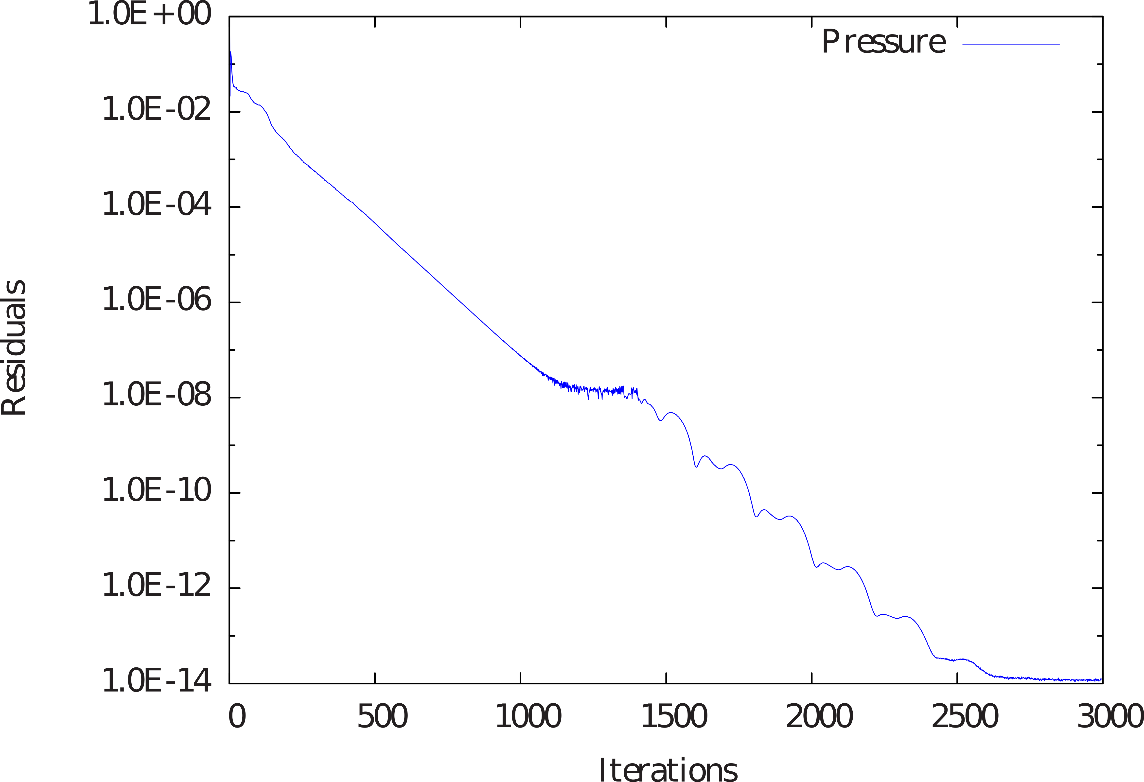
Figure 9 Convergence of pressure with respect to number of iterations.
Results
The solution obtained for the tee-junction at steady state is shown here using qualitative contour plots. In Figure 10, velocity magnitude and pressure contour plots are shown. In addition, streamlines superimposed on the velocity magnitude is given. The change in the flow pattern due to the presence of side branch is quite evident from the velocity magnitude contour. The streamlines particularly facilitate to visualise the flow separation phenomenon which is occurring in this case, just before the flow entering the side branch. Also to note is the velocity profile at the inlet, which is fully developed as expected.
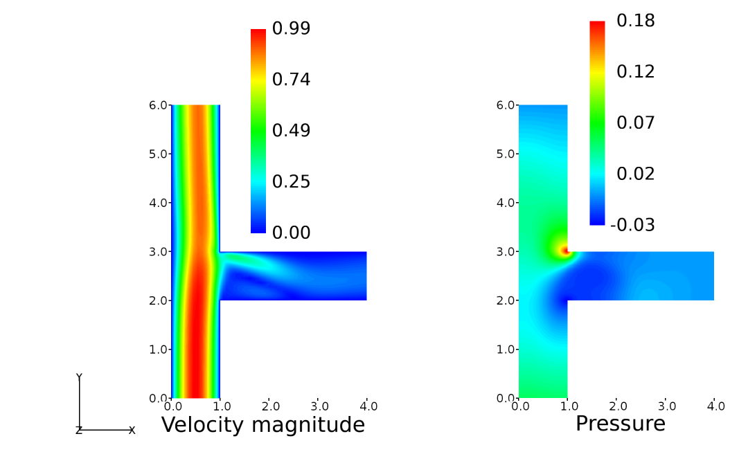
Figure 10 Velocity magnitude and pressure contour plots within the tee-junction
Circular Cylinder
The simulation of laminar, incompressible flow over a two-dimensional circular cylinder is shown in this tutorial. Caelus 9.04 will be used and the details of setting up directory structure, fluid properties, boundary conditions, etc will be shown. This tutorial introduces to the user in carrying out a time-dependent simulation of a externally separated flow. Further to this, the flow around the cylinder would be visualised using velocity and pressure contours.
Objectives
Through this tutorial, the user would be familiar in setting up a time-dependent Caelus simulation for laminar, incompressible flow in two-dimensions for external separated flows. Following will be some of the steps that will be performed.
- Background
A brief description about the problem
Geometry and freestream details
- Grid generation
Computational domain and boundary details
Computational grid generation
Exporting grid to Caelus
- Problem definition
Directory structure
Setting up boundary conditions, physical properties and control/solver attributes
- Execution of the solver
Monitoring the convergence
Writing the log files
- Results
Showing the flow structure in near and far wake
Pre-requisites
It is assumed that the user is familiar with the Linux command line environment using a terminal or Caelus-console (for Windows OS) and that Caelus is installed correctly with appropriate environment variables set. The grid used here is generated using Pointwise and the user is free to use their choice of grid generation tool having exporting capabilities to the Caelus grid format.
Background
The flow over a circular cylinder is a classical configuration to study separation and its related phenomena. This provides an ideal case for the user to use Caelus for flow over bluff bodies that represents externally separated flow. It has been shown that for low Reynolds number flows (\(40 \leq Re \leq 150\)), period vortex shedding occurs in the wake. This phenomena of vortex shedding behind bluff bodies is referred as the Karman Vortex Street [2]. The frequency associated with the oscillations of vortex streets can be expressed via Strouhal number (\(St\)) which is non-dimensional relating to the frequency of oscillations (\(f\)) of vortex shedding, cylinder diameter (\(D\)) and the flow velocity (\(U\)) as
For a Reynolds number based on the cylinder diameter of \(Re_D = 100\), the Strouhal number is about \(St\approx 0.16-0.17\) as determined through experiments and is nearly independent of the diameter of the cylinder. More details are discussed in section Circular Cylinder
The diameter chosen for the cylinder here is \(D = 2~m\) and is the characteristic length for the Reynolds number, which is (\(Re_D = 100\)). The velocity is assumed to be \(U = 1~m/s\) in the \(x\) direction. Based on these, the kinematic velocity can be estimated as \(\nu = 0.02~m^2/s\). The below Figure 11 shows the schematic of the cylinder in the \(x-y\) plane.

Figure 11 Schematic of the circular cylinder in two-dimensions
In the below table a summary of the freestream conditions are given
\(Re_D\) |
\(U~(m/s)\) |
\(p~(m^2/s^2)\) |
\(\nu~(m^2/s)\) |
|---|---|---|---|
100 |
1.0 |
\((0)\) Gauge |
\(0.02\) |
Grid Generation
A hexahedral grid around the circular cylinder was development with a O-grid topology using Pointwise. Specific grid generation details are omitted while proving sufficient details regarding computational domain and boundary conditions. With these details the user should be able to recreate the required grid for the two-dimensional cylinder
A rectangular computational domain in the \(x-y\) plane has been constructed surrounding the circular cylinder as shown in Figure 12. A full cylinder was considered as the vortices developed behind the cylinder are of the periodic nature. Upstream of the cylinder, the domain is extended by 5 cylindrical diameters, whereas, downstream it was extended up to 20. Since the flow here is viscous dominated, sufficient downstream length is required to capture the initial vortex separation from the surface of the cylinder and the subsequent shedding process. In the \(y\) direction, the domain is extended up to 5 cylindrical diameters on either side. From the figure, multiple inlet boundaries to this domain can be seen, one at the far end of the upstream and the other two for the top and bottom boundaries. This type of configuration is particularly needed to appropriately model the inflow, very similar to an undisturbed flow in an experimental set-up. It should be noted here that for top and bottom boundaries, the flow is in the \(x\) direction. Outlet boundary to the domain is placed at the downstream end which is at 20 cylindrical diameters. Since the fluid behaviour is viscous, the velocity at the wall is zero (\(u, v, w = 0~m/s\)) represented here through a no-slip boundary condition as highlighted in blue.

Figure 12 Circular cylinder computational domain
The hexahedral grid around the cylinder is shown in Figure 13 for a \(x-y\) plane. Caelus is a 3D solver and requires the grid to be in 3D. This was obtained by extruding the grid in the \(x-y\) plane by one cell thick and subsequently specifying empty boundary conditions to the extruded planes. This enforces that Caelus to solve the flow in two dimensions assuming symmetry in the \(z\) direction as is required in this case due to the two-dimensionality of the flow.
Note
A velocity value of \(w=0\) needs to be specified at appropriate boundaries although no flow is solved in the \(z\) direction.
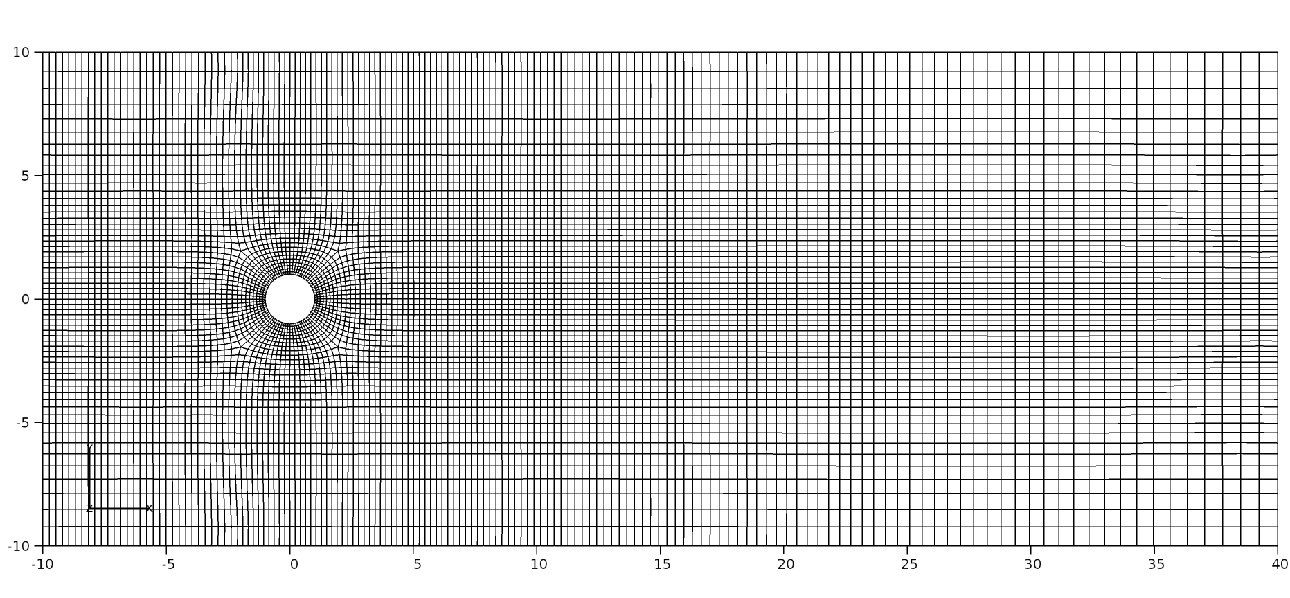
Figure 13 O-grid around the cylinder and structured gird representation
The 2D domain consisted of 9260 cells in total. An O-grid topology is constructed around the cylinder and extended to a maximum of 1 cylindrical diameter in the radial direction with a distribution of 10 cells. Around the cylinder, 84 cells are used giving 21 cells per each O-grid block. Upstream of the O-grid in the \(x\) direction, 31 cells were used and 100 in the downstream. The region of interest is about 10 diameters downstream, where the grids are refined. In the \(y\) direction, both positive and negative axes, 21 cells are used beyond the O-grid region.
Problem definition
We first begin with instructions to set-up the circular cylinder case in addition to the configuration files that are needed. A full working case can be found in the following directory:
/tutorials/incompressible/pimpleSolver/laminar/ACCM_circularCylinder/
However, the user is free to start the case setup from scratch consistent with the directory stucture discussed below.
Directory Structure
Note
All commands shown here are entered in a terminal window, unless otherwise mentioned
For setting up this problem, Caelus requires time, constant and system sub-directories within the main working directory. Since we start the simulation at time, t = 0 s, a time sub-directory named 0 is required.
The 0 sub-directory contains files, p and U, which describe the dimensions, initialisation and boundary conditions of pressure (\(p\)) and velocity (\(U\)) respectively.
It is to be noted that Caelus is case sensitive and therefore the user should set-up the directories (if applicable), files and the contents identical to what is mentioned here.
Boundary Conditions
We now begin with setting up the boundary conditions. Referring back to Figure 12, the following are the boundary conditions that need to be specified:
- Inlet
Velocity: Fixed uniform velocity \(u = 1.0~m/s\) in \(x\) direction
Pressure: Zero gradient
- No-slip wall
Velocity: Fixed uniform velocity \(u, v, w = 0\)
Pressure: Zero gradient
- Outlet
Velocity: Zero gradient velocity
Pressure: Fixed uniform gauge pressure \(p = 0\)
- Initialisation
Velocity: Fixed uniform velocity \(u = 1.0~m/s\) in \(x\) direction
Pressure: Zero Gauge pressure
Beginning with the pressure (\(p\)), the dictionary begins with FoamFile containing standard set of keywords for version, format, location, class and object names as shown below.
/*-------------------------------------------------------------------------------*
Caelus 9.04
Web:   www.caelus-cml.com
\*------------------------------------------------------------------------------*/

FoamFile
{
	version				2.0;
	format				ascii;
	class				volScalarField;
	object				p;
}

//--------------------------------------------------------------------------------

dimensions				[0 2 -2 0 0 0 0];

internalField				uniform 0;

boundaryField
{
	inlet-1
	{
		type			zeroGradient;
	}
	inlet-2
	{
		type			zeroGradient;
	}
	outlet
	{
		type			fixedValue;
		value			uniform 0;
	}
	symmetry
	{
		type			empty;
	}
	wall
	{
		type			zeroGradient;
	}
}
The following provides the explanation to the principle entries
dimensionis used to specify the physical dimensions of the pressure field. Here, pressure is defined in terms of kinematic pressure with the units (\(m^2/s^2\)) written as
[0 2 -2 0 0 0 0]
internalFieldis used to specify the initial conditions. It can be either uniform or non-uniform. Since we have a 0 initial uniform gauge pressure, the entry is
uniform 0
boundaryFieldis used to specify the boundary conditions. In this case its the boundary conditions for pressure at all the boundary patches.
In a similar manner, the file U contains the following entries
/*-------------------------------------------------------------------------------*
Caelus 9.04
Web:   www.caelus-cml.com
\*-------------------------------------------------------------------------------*/

FoamFile
{
	version				2.0;
	format				ascii;
	class				volVectorField;
	object				U;
}

//--------------------------------------------------------------------------------

dimensions				[0 1 -1 0 0 0 0];

internalField				uniform (1.0 0 0);

boundaryField
{
	inlet-1
	{
		type			fixedValue;
		value			uniform (1.0 0 0);
	}
	inlet-2
	{
		type			fixedValue;
		value			uniform (1.0 0 0);
	}
	outlet
	{
		type			zeroGradient;
	}
	symmetry
	{
		type			empty;
	}
	wall
	{
		type			fixedValue;
		value			uniform (0 0 0);
	}
}
The principle entries for velocity field are self explanatory and the dimension are typical for velocity with the units \(m/s\) ([0 1 -1 0 0 0 0]). Since we initialise the flow with a uniform freestream velocity, we set the internalField to uniform (1.0 0 0) representing three components of velocity. Similarly, inlets and wall boundary patches have three velocity components.
Before proceeding further, it is important to ensure that the boundary conditions (inlet, outlet, wall, etc) specified in the above files should be the grid boundary patches (surfaces) generated by the grid generation tool and their names are identical. Further, the two boundaries in \(x-y\) plane obtained due to grid extrusion have been named as symm-left and symm-right with specifying empty boundary conditions forcing Caelus to assume the flow to be in two-dimensions. This completes the setting up of boundary conditions.
Grid file and Physical Properties
The circular cylinder grid file is placed in the constant/polyMesh sub-directory. Additionally, the physical properties are specified in different files present in the constant directory.
The first file is transportProperties, where the transport model and the kinematic viscosity are specified. The contents of this file are as follows
/*-------------------------------------------------------------------------------*
Caelus 9.04
Web:   www.caelus-cml.com
\*------------------------------------------------------------------------------*/

FoamFile
{
	version				2.0;
	format				ascii;
	class				dictionary;
	location			"constant";
	object				transportProperties;
}

//--------------------------------------------------------------------------------

transportModel				Newtonian;

nu					nu [0 2 -1 0 0 0 0] 0.02;
Since the flow is Newtonian, the transportModel is specified with Newtonian keyword and the value of kinematic viscosity (nu) is given which has the units \(m^2/s\) ([0 2 -1 0 0 0 0]).
The final in this sun-directory is the turbulenceProperties file, where the type of simulation is specified as
/*-------------------------------------------------------------------------------*
Caelus 9.04
Web:   www.caelus-cml.com
\*------------------------------------------------------------------------------*/
FoamFile
{

	version				2.0;
	format				ascii;
	class				dictionary;
	location			"constant";
	object				turbulenceProperties;
}

//--------------------------------------------------------------------------------

simulationType				laminar;
As the flow here is laminar, the simulationType would be laminar.
Controls and Solver Attributes
This section details the files required to control the simulation, specifying the type of discretization method and linear solver settings. These files can be found in the system directory.
The first file, controlDict is shown below
/*-------------------------------------------------------------------------------*
Caelus 9.04
Web:   www.caelus-cml.com
\*------------------------------------------------------------------------------*/

FoamFile
{
	version				2.0;
	format				ascii;
	class				dictionary;
	location			"system";
	object				controlDict;
}

//--------------------------------------------------------------------------------

application				pimpleSolver;

startFrom				startTime;

startTime				0;

stopAt					endTime;

endTime					360;

deltaT					0.01;

writeControl			runTime;

writeInterval			1;

purgeWrite				0;

writeFormat				ascii;

writePrecision			6;

writeCompression		uncompressed;

timeFormat				general;

timePrecision			6;

runTimeModifiable		true;

//-------------------------------------------------------------------------------

// Function Objects to obtain mean values

functions
{
	forces
	{
        type                forces;
        functionObjectLibs	("libforces.so");
        patches             ( wall );
        CofR                (0 0 0);
        rhoName             rhoInf;
        rhoInf              1;
        writeControl        timeStep;
        writeInterval       50;
     }
}
//------------------------------------------------------------------------------
In this file, the application pimpleSolver refers to the PIMPLE solver that is used in this tutorial. We also begin the simulation at t = 0 s, which logically explains the need for 0 directory where the data files are read at the beginning of the run. Therefore, we need to set the keyword startFrom to startTime, where startTime would be 0. The simulation is run for 360 seconds specifying through the keywords stopAt and endTime. Since PIMPLE solver is time-accurate, we also need to set the time-step via deltaT. The results are written at every 0.01 seconds via writeControl and writeInterval keywords.
The discretization schemes and its parameters are specified in the fvSchemes file which is shown below
/*-------------------------------------------------------------------------------*
Caelus 9.04
Web:   www.caelus-cml.com
\*------------------------------------------------------------------------------*/
FoamFile
{
	version				2.0;
	format				ascii;
	class				dictionary;
	object				fvSchemes;
}

//--------------------------------------------------------------------------------

ddtSchemes
{
	default				Euler;
}

gradSchemes
{
	default				Gauss	linear;
	grad(p)				Gauss	linear;
	grad(U)				Gauss	linear;
}

divSchemes
{
	default				none;
	div(phi,U)			Gauss	linearUpwindBJ grad(U);
	div((nuEff*dev(T(grad(U)))))	Gauss   linear;
}

laplacianSchemes
{
	default				none;
	laplacian(nu,U)			Gauss 	linear 	corrected;
	laplacian(nuEff,U)		Gauss 	linear 	corrected;
	laplacian(p)			Gauss	linear 	corrected;
	laplacian((1|A(U)),p)           Gauss   linear  corrected;
	laplacian(rAUf,p)               Gauss   linear  corrected;

}

interpolationSchemes
{
	default				linear;
	interpolate(HbyA)		linear;
}

snGradschemes
{
	default				corrected;
}
In the fvSolution file, linear solver controls and tolerances are set as shown in the below file
/*-------------------------------------------------------------------------------*
Caelus 9.04
Web:   www.caelus-cml.com
\*------------------------------------------------------------------------------*/

FoamFile
{
	version				2.0;
	format				ascii;
	class				dictionary;
	location			"system";
	object				fvSolution;
}

//--------------------------------------------------------------------------------

solvers
{
	p
	{
		solver			PCG;
		preconditioner		SSGS;
		tolerance		1e-6;
		relTol			0.05;
	}
	pFinal
	{
		solver			PCG;
		preconditioner		SSGS;
		tolerance		1e-7;
		relTol			0;
	}
	UFinal
	{
		solver			PBiCGStab;
		preconditioner		USGS;
		tolerance		1e-6;
		relTol			0;
	}
	U
	{
		solver			PBiCGStab;
		preconditioner		USGS;
		tolerance		1e-6;
		relTol			0;
	}
}

PIMPLE
{
	nCorrectors                     2;
	nNonOrthogonalCorrectors	1;
	pRefCell			0;
	pRefValue			0;
}
Note that different linear solvers are used here to solve for pressure and velocity. Also, nNonOrthogonalCorrectors is set to 1, since there is some degree of non-orthogonality in the grid.
At this stage, the directory structure should be identical to the one shown below. This can be done by using the tree command on Linux OS.
tree
.
├── 0
│   ├── p
│   └── U
├── constant
│   ├── polyMesh
│   │   ├── boundary
│   │   ├── faces
│   │   ├── neighbour
│   │   ├── owner
│   │   ├── points
│   │   └── sets
│   ├── transportProperties
│   └── turbulenceProperties
└── system
    ├── controlDict
    ├── fvSchemes
    └── fvSolution
Execution of the solver
Prior to solver execution, renumbering of the grid or mesh needs to be performed as well as checking the quality of the grid. Renumbering the grid-cell list is vital to reduce the matrix bandwidth while the quality check gives us the mesh statistics. Renumbering and mesh quality can be determined by executing the following from the top directory
caelus run -- renumberMesh -overwrite
caelus run -- checkMesh
The user should take note of the bandwidth before and after the mesh renumbering. When the checkMesh is performed, the mesh statistics are shown as below
/*---------------------------------------------------------------------------*\
 Caelus 8.04
 Web:      www.caelus-cml.com
\*---------------------------------------------------------------------------*/

Checking geometry...
    Overall domain bounding box (-10 -10 0) (40 10 0.537713)
    Mesh (non-empty, non-wedge) directions (1 1 0)
    Mesh (non-empty) directions (1 1 0)
    All edges aligned with or perpendicular to non-empty directions.
    Boundary openness (-2.57817e-19 1.67414e-19 -4.29222e-16) OK.
    Max cell openness = 2.19645e-16 OK.
    Max aspect ratio = 3.66844 OK.
    Minimum face area = 0.00895343. Maximum face area = 0.586971.  Face area magnitudes OK.
    Min volume = 0.00481437. Max volume = 0.315622.  Total volume = 536.025.  Cell volumes OK.
    Mesh non-orthogonality Max: 14.6136 average: 1.75565
    Non-orthogonality check OK.
    Face pyramids OK.
    Mesh skewness Max: 0.206341 average: 0.00112274 OK.
    Coupled point location match (average 0) OK.

Mesh OK.
In the next step, execution of the solver can be performed while monitoring the progress of the solution. The solver is always executed from the top directory which is ACCM_circularCylinder in this case.
caelus run -l my-circular-cylinder.log -- pimpleSolver
The output of the solution process is saved in the log file, my-circular-cylinder.log. In a separate terminal window the convergence history can be monitored using
caelus logs -w my-circular-cylinder.log
With the above, the convergence of pressure along with other variables can be seen with respect to time. The same is shown in the Figure 14 and due to the periodic nature of vortex shedding, oscillatory convergence of pressure is seen.
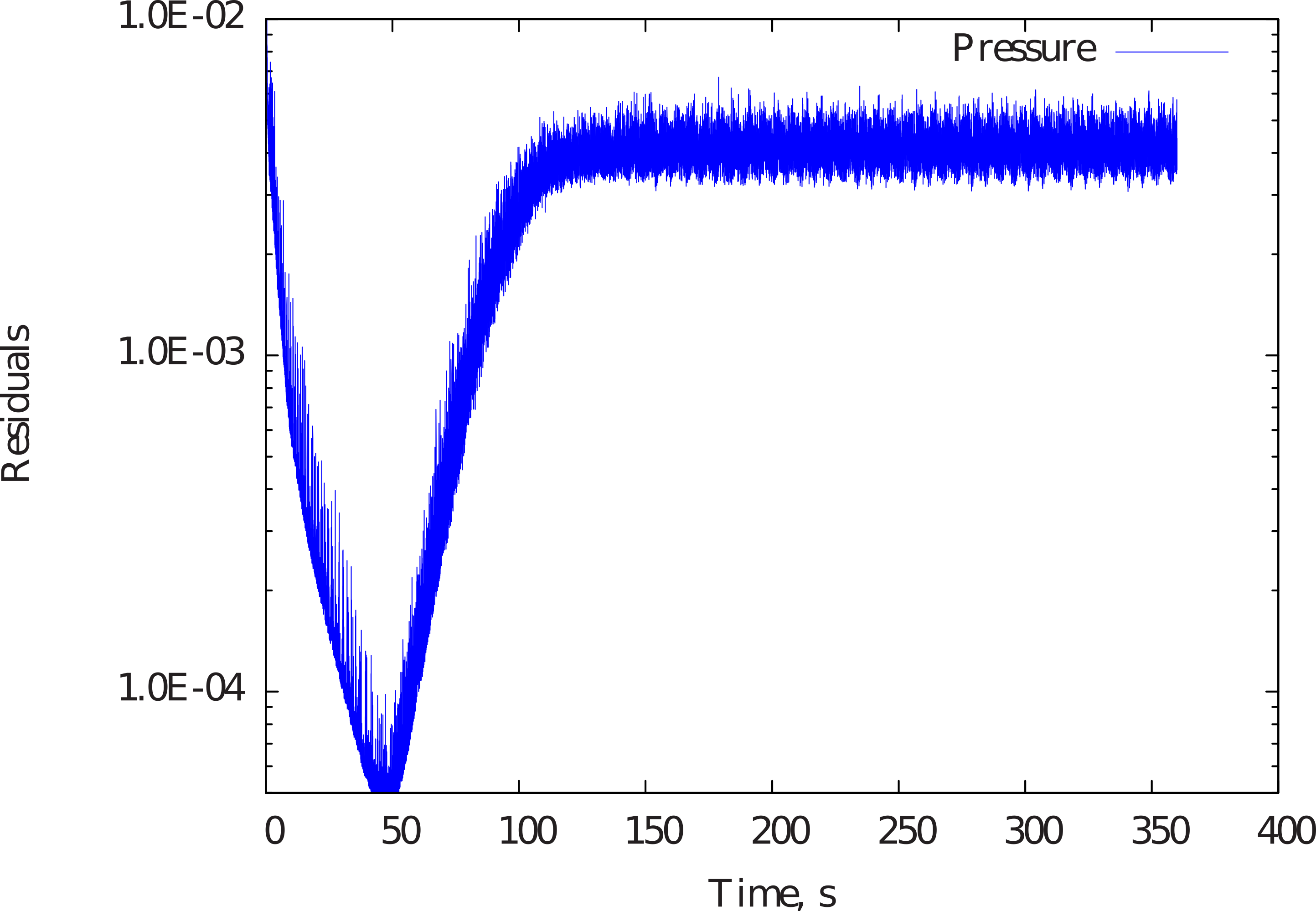
Figure 14 Convergence of pressure with respect to time
Results
In this section, some qualitative results obtained as a result of steady vortex shedding in the wake of the cylinder is shown. Figure 15 shows the velocity magnitude and pressure contour for the flow over the cylinder. The formation of vortex shedding is clearly visible from the velocity contour and the pressure variation due to oscillating vortex in the wake. The vortex break-up that occurs in the near wake of the cylinder, travels several diameters downstream eventually diffusing into the flow.
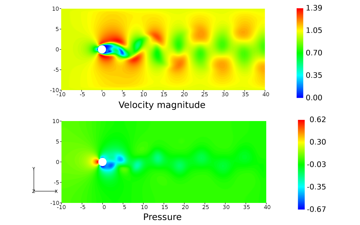
Figure 15 Velocity magnitude and pressure contour plots for the flow over the 2D cylinder
Triangular Cavity
In this tutorial, we carry out laminar, incompressible flow inside a triangular cavity in two-dimensions using Caelus 9.04. Details regarding setting up of the directories, fluid properties, boundary conditions, etc will be discussed. Subsequent to this, post-processing the velocity distribution along the center-line will be shown.
Objectives
With the completion of this tutorial, the user would be familiar with setting up a steady-state Caelus simulation for laminar, incompressible flow over lip-driven cavity. Following are the steps that would be performed
- Background
A brief description about the problem
Geometry and freestream details
- Grid generation
Computational domain and boundary details
Computational grid generation
Exporting grid to Caelus
- Problem definition
Directory structure
Setting up boundary conditions, physical properties and control/solver attributes
- Execution of the solver
Monitoring the convergence
Writing the log files
- Results
Showing the flow structure inside the cavity
Pre-requisites
It is assumed that the user is familiar with the Linux command line environment using a terminal or Caelus-console (for Windows OS) and that Caelus is installed correctly with appropriate environment variables set. The grid used here is generated using Pointwise and the user is free to use their choice of grid generation tool having exporting capabilities to the Caelus grid format.
Background
Flow inside lid-driven cavities is a classical case to study cases with flow recirculation. In the present case, the top wall of the cavity moves at constant velocity initiating a recirculation motion with the cavity and as a consequence, a boundary layer develops in the direction of the moving lid. The feature that is of interest is the velocity distribution along the center-line of cavity. Details regarding the validation of this case is given in Triangular Cavity.
The triangular cavity schematic is shown in Figure 16. Here D represents the cavity depth which is 4 m and the top width, W = 2 m. For this configuration, the Reynolds number based on the cavity depth is 800 and the wall velocity is assumed and set to 2 m/s. This give us with a kinematic viscosity of 0.01. Note that the two-dimensional plane considered here is in \(x-z\).
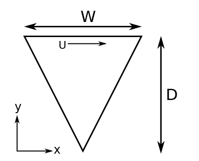
Figure 16 Schematic of a triangular cavity
The below table gives the summary of the freestream conditions used here
\(Re_D\) |
\(U~(m/s)\) |
\(p~(Pa)\) |
\(\nu~(m^2/s)\) |
|---|---|---|---|
800 |
2.0 |
\((0)\) Gauge |
\(0.01\) |
Grid Generation
A hybrid-grid consisting of quadrilateral and triangular cells has been generated for this cavity geometry using Pointwise. Details regarding the generation of grid is not covered in this tutorial, however details regarding computational domain and boundary conditions are provided.
The computational domain for the triangular cavity follows the cavity geometry due to internal flow configuration. This is in contrast to other flow configurations here where the flow was over the region of interest. A schematic of the domain is shown in Figure 17. The velocity at the cavity walls (high lighted in blue) is zero, represented through a no-slip boundary, wherein \(u, v, w = 0\). Whereas the top wall has a uniform velocity in the x-direction.

Figure 17 Computational domain for a triangular cavity
The hybrid grid is shown in Figure 18. As can be seen, up to a depth of D = 1.35 m, structured grids are used and after which it is filled with triangular unstructured elements. In the structured domain, 40 X 40 cells are used respectively. In the 2D domain, a total of 5538 cells are present, however the polyMesh format of Caelus should be in 3D. This was achieved by extruding the grid in the \(x-y\) plane by one cell thick and subsequently specifying empty boundary conditions to the extruded planes. This should force Caelus to solve the flow the flow in 2D in the extruded direction, which is \(z\).
Note
A velocity value of \(w=0\) needs to be specified at appropriate boundaries although no flow is solved in the \(z\) direction.
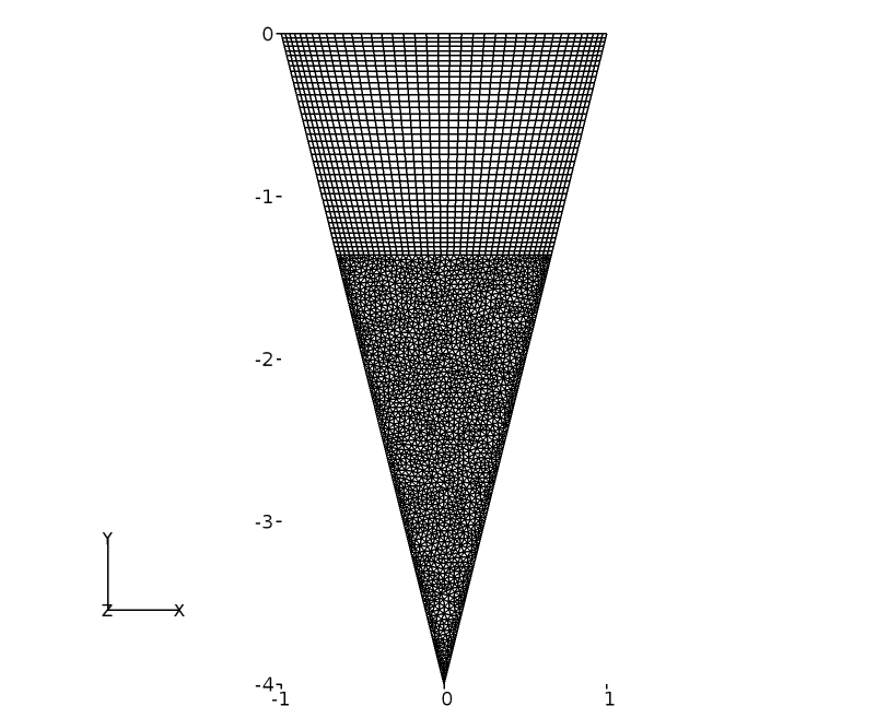
Figure 18 Hybrid grid representation for a triangular cavity
Problem definition
This section provides the case set-up procedures along with the configuration files that are needed. A full working case of this problem is given in the following location:
/tutorials/incompressible/pimpleSolver/laminar/ACCM_triangularCavity/
However,the user is free to start the case setup from scratch consistent with the directory stucture discussed below.
Directory Structure
Note
All commands shown here are entered in a terminal window, unless otherwise mentioned
Caelus requires time, constant and system sub-directories within the main my-triangular-cavity working directory. Since we start the simulation at time, t = 0 s, a time sub-directory named 0 is required.
The 0 sub-directory contains the pressure, p and velocity U files. The contents of these files set the dimensions, initialisation and boundary conditions to the case, which form the three principle entries required.
If applicable, the user should take precautions in setting the directories and files as Caelus is case sensitive. These have to be identical to the names mentioned here.
Boundary Conditions
Next we start with setting-up of the boundary conditions. Referring back to Figure 17, the following are the boundary conditions that need to be specified:
- Moving wall
Velocity: Fixed uniform velocity \(u = 2.0~m/s\) in \(x\) direction
Pressure: Zero gradient
- No-slip wall
Velocity: Fixed uniform velocity \(u, v, w = 0\)
Pressure: Zero gradient
- Initialisation
Velocity: Fixed uniform velocity \(u = 0~m/s\) in \(x, y, z\) directions
Pressure: Zero Gauge pressure
The file p for pressure contains the following information
/*-------------------------------------------------------------------------------*
Caelus 9.04
Web:   www.caelus-cml.com
\*------------------------------------------------------------------------------*/

FoamFile
{
	version				2.0;
	format				ascii;
	class				volScalarField;
	object				p;
}

//--------------------------------------------------------------------------------

dimensions				[0 2 -2 0 0 0 0];

internalField				uniform 0;

boundaryField
{
	fixed-walls
	{
		type			zeroGradient;
	}
	moving-wall
	{
		type			zeroGradient;
	}
    symm
	{
		type			empty;
	}
}
As noted from the above file, the dictionary begins with FoamFile containing standard set of keywords for version, format, location, class and object names. The following provides the explanation to the principle entries
dimensionis used to specify the physical dimensions of the pressure field. Here, pressure is defined in terms of kinematic pressure with the units (\(m^2/s^2\)) written as
[0 2 -2 0 0 0 0]
internalFieldis used to specify the initial conditions. It can be either uniform or non-uniform. Since we have a 0 initial uniform gauge pressure, the entry is
uniform 0
boundaryFieldis used to specify the boundary conditions. In this case its the boundary conditions for pressure at all the boundary patches.
Similarly, the contents for the file U is as shown below
/*-------------------------------------------------------------------------------*
Caelus 9.04
Web:   www.caelus-cml.com
\*------------------------------------------------------------------------------*/
FoamFile
{
	version				2.0;
	format				ascii;
	class				volVectorField;
	location			"0";
	object				U;
}

//--------------------------------------------------------------------------------

dimensions				[0 1 -1 0 0 0 0];

internalField				uniform (0 0 0);

boundaryField
{
	fixed-walls
	{
		type            	fixedValue;
        value				uniform (0 0 0);
	}
	moving-wall
	{
		type            	fixedValue;
        value				uniform (2 0 0);
	}
    symm
	{
		type			empty;
	}
}
The principle entries for velocity field are self explanatory and the dimension are typical for velocity with the units \(m/s\) ([0 1 -1 0 0 0 0]). Here, since the top wall moves with a velocity, we set a uniform (2.0 0 0) for moving-wall boundary patch. Similarly, the cavity walls (fixed-walls) have uniform (1.0 0 0).
At this stage, the user should ensure that the boundary conditions (fixed-walls, moving-wall and symm) specified in the above files should be the grid boundary patches (surfaces) generated by the grid generation tool and their names are identical. Further, the two boundaries in \(x-y\) plane obtained due to grid extrusion have been combined and named as symm with specifying empty boundary conditions forcing Caelus to assume the flow to be in two-dimensions. With this, the setting up of boundary conditions are completed.
Grid file and Physical Properties
The triangular cavity grid is placed in constant/polyMesh sub-directory. In addition, the physical properties are specified in different files, all present in the constant directory.
The transport model and the kinematic viscosity are specified in the file transportProperties. The contents of this file are as follows
/*-------------------------------------------------------------------------------*
Caelus 9.04
Web:   www.caelus-cml.com
\*------------------------------------------------------------------------------*/

FoamFile
{
	version				2.0;
	format				ascii;
	class				dictionary;
	location			"constant";
	object				transportProperties;
}

//--------------------------------------------------------------------------------

transportModel				Newtonian;

nu					nu [0 2 -1 0 0 0 0] 0.01;
Since the viscous behaviour is modelled as Newtonian, the transportModel is specified with the keyword Newtonian and the value of kinematic viscosity is set with has the units \(m^2/s\) ([0 2 -1 0 0 0 0]).
The final file in this class is the turbulenceProperties file, in which the type of simulation is specified as
/*-------------------------------------------------------------------------------*
Caelus 9.04
Web:   www.caelus-cml.com
\*------------------------------------------------------------------------------*/

FoamFile
{

	version				2.0;
	format				ascii;
	class				dictionary;
	location			"constant";
	object				turbulenceProperties;
}

//--------------------------------------------------------------------------------

simulationType				laminar;
The flow being laminar, the simulationType is set to laminar.
Controls and Solver Attributes
In this section, the files required to control the simulation, setting the discretization parameters and linear solver settings are discussed can be found in the system directory.
The controlDict file is shown below.
/*-------------------------------------------------------------------------------*
Caelus 9.04
Web:   www.caelus-cml.com
\*------------------------------------------------------------------------------*/

FoamFile
{
	version				2.0;
	format				ascii;
	class				dictionary;
	location			"system";
	object				controlDict;
}

//-------------------------------------------------------------------------------

application				pimpleSolver;

startFrom				startTime;

startTime				0;

stopAt					endTime;

endTime					60;

deltaT					0.01;

writeControl				runTime;

writeInterval				1;

purgeWrite				0;

writeFormat				ascii;

writePrecision				6;

writeCompression			uncompressed;

timeFormat				general;

timePrecision				6;

runTimeModifiable			true;
In the controlDict file, pimpleSolver refers to the application, PIMPLE solver that is used here. The simulation is also started at t = 0 s and this logically explains the need for 0 directory where the data files are read at the beginning of the run. Therefore, the keyword startFrom to startTime, where startTime would be 0 is needed. The simulation is run for 200 seconds specifying through the keywords stopAt and endTime. Since PIMPLE solver is time-accurate, we also need to set the time-step via deltaT. The results are written at every 0.01 seconds via writeControl and writeInterval keywords.
The discretization schemes and its parameters are specified in the fvSchemes file which is shown below
/*-------------------------------------------------------------------------------*
Caelus 9.04
Web:   www.caelus-cml.com
\*------------------------------------------------------------------------------*/

FoamFile
{
	version				2.0;
	format				ascii;
	class				dictionary;
	object				fvSchemes;
}

//--------------------------------------------------------------------------------

ddtSchemes
{
	default				Euler;
}

gradSchemes
{
	default				Gauss	linear;
	grad(p)				Gauss	linear;
	grad(U)				Gauss	linear;
}

divSchemes
{
	default				none;
	div(phi,U)			Gauss	linearUpwindBJ grad(U);
	div((nuEff*dev(T(grad(U)))))	Gauss   linear;
}

laplacianSchemes
{
	default				none;
	laplacian(nu,U)			Gauss 	linear 	corrected;
	laplacian(nuEff,U)		Gauss 	linear 	corrected;
	laplacian(p)			Gauss 	linear 	corrected;
	laplacian((1|A(U)),p)           Gauss   linear  corrected;
	laplacian(rAUf,p)		Gauss 	linear 	corrected;

}

interpolationSchemes
{
	default				linear;
	interpolate(HbyA)		linear;
}

snGradschemes
{
	default				corrected;
}
In the following file, which is the fvSolution the linear solver controls and tolerances are set as shown below
/*-------------------------------------------------------------------------------*
Caelus 9.04
Web:   www.caelus-cml.com
\*------------------------------------------------------------------------------*/

FoamFile
{
	version				2.0;
	format				ascii;
	class				dictionary;
	location			"system";
	object				fvSolution;
}

//------------------------------------------------------------------------------

solvers
{
	p
	{
		solver			PCG;
		preconditioner		SSGS;
		tolerance		1e-10;
		relTol			0;
	}
	pFinal
	{
		solver			PCG;
		preconditioner		SSGS;
		tolerance		1e-10;
		relTol			0;
	}
	UFinal
	{
		solver			PBiCGStab;
		preconditioner		USGS;
		tolerance		1e-15;
		relTol			0;
	}
	U
	{
		solver			PBiCGStab;
		preconditioner		USGS;
		tolerance		1e-15;
		relTol			0;
	}
}

PIMPLE
{
	nCorrectors                     2;
	nNonOrthogonalCorrectors	1;
	pRefCell			0;
	pRefValue			0;
}
It should be noted that different linear solvers are used to solve for pressure a velocity. Since we have used hybrid grids, nNonOrthogonalCorrectors is set to 1 as there would be some degree of non-orthogonality present due to triangular nature of the geometry.
This completes the set-up of directory structure along with all the necessary files. This can be verified by using the following commands and the directory tree should be identical to the one shown below
tree
.
├── 0
│   ├── p
│   └── U
├── constant
│   ├── polyMesh
│   │   ├── boundary
│   │   ├── faces
│   │   ├── neighbour
│   │   ├── owner
│   │   └── points
│   ├── transportProperties
│   └── turbulenceProperties
└── system
    ├── controlDict
    ├── fvSchemes
    ├── fvSolution
Execution of the solver
Renumbering and checking the mesh quality is needed before the solver is executed. Renumbering the grid-cell list is vital to reduce the matrix bandwidth while the quality check gives us the mesh statistics. Renumbering and mesh quality can be determined by executing the following from the top directory
caelus run -- renumberMesh -overwrite
caelus run -- checkMesh
The user should take note of the bandwidth before and after the mesh renumbering. When the checkMesh is performed, the mesh statistics are shown as below
/*---------------------------------------------------------------------------*\
 Caelus 8.04
 Web:      www.caelus-cml.com
\*---------------------------------------------------------------------------*/

Checking geometry...
    Overall domain bounding box (-1 -4 0) (1 0 0.0447214)
    Mesh (non-empty, non-wedge) directions (1 1 0)
    Mesh (non-empty) directions (1 1 0)
    All edges aligned with or perpendicular to non-empty directions.
    Boundary openness (-6.25534e-18 -5.30678e-18 -6.4712e-16) OK.
    Max cell openness = 2.16191e-16 OK.
    Max aspect ratio = 2.97779 OK.
    Minimum face area = 8.00174e-05. Maximum face area = 0.00322809.  Face area magnitudes OK.
    Min volume = 3.57849e-06. Max volume = 0.000109372.  Total volume = 0.178886.  Cell volumes OK.
    Mesh non-orthogonality Max: 41.8682 average: 9.34065
    Non-orthogonality check OK.
    Face pyramids OK.
    Mesh skewness Max: 0.621726 average: 0.0313562 OK.
    Coupled point location match (average 0) OK.

Mesh OK.


End
Solver can now be executed and the progress of the solution can be monitored. The solver is always executed from the top directory which is my-triangular-cavity in this case.
caelus run -l my-triangular-cavity.log pimpleSolver
The output of the solver progress is saved in the log file, my-triangular-cavity.log. The log file (my-triangular-cavity.log) can be monitored to look at the convergence history. In a separate terminal window use
caelus logs -w my-triangular-cavity.log
The convergence of the pressure can now be seen with respect to time.
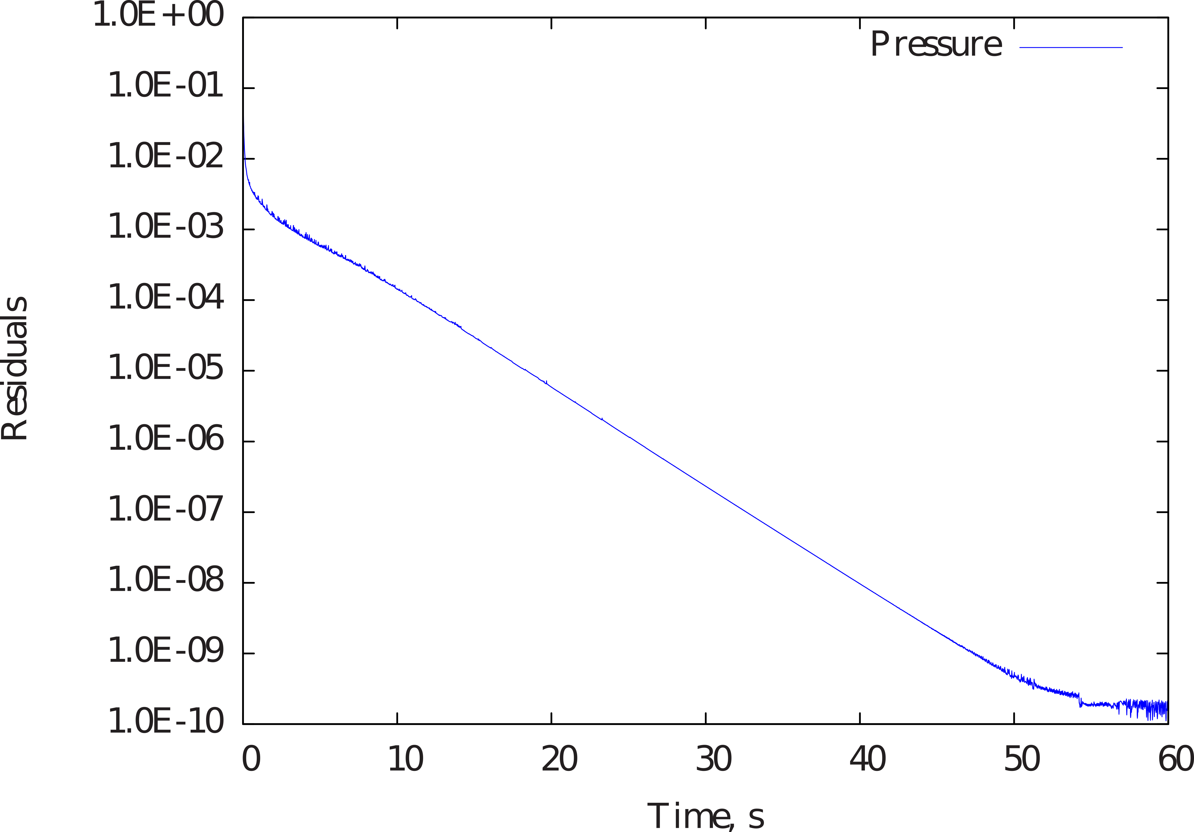
Figure 19 Convergence of pressure with respect to time
Results
The flow within the cavity is shown here at steady state condition. Figure 20 presents the velocity and pressure contour plots. In addition, the streamlines indicate the multiple vortices formed within the cavity.
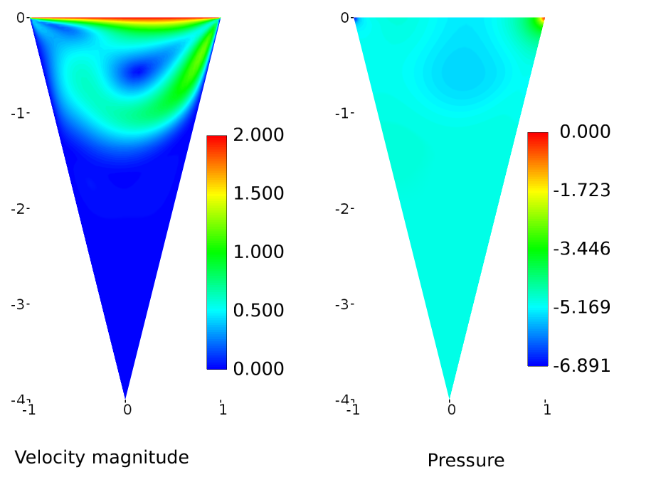
Figure 20 Velocity magnitude and pressure contour plots within the triangular cavity
Spherical Cavity
In this tutorial, we look at simulating buoyant flow inside a spherically heated cavity using Caelus 9.04 which will be a three-dimension case. Because of the natural convection process, the fluid initiates a motion due to buoyancy effects. This results in steady isotherms which is of interest in this tutorial and will be compared with the analytical data.
Objectives
With this tutorial, the user would be familiar in setting up a steady-state Caelus simulation for laminar, buoyant flow within a spherically heated cavity. The steps that would be performed in this tutorial are as follows
- Background
A brief description about the problem
Geometry and freestream details
- Grid generation
Computational domain and boundary details
Computational grid generation
Exporting grid to Caelus
- Problem definition
Directory structure
Setting up boundary conditions, physical properties and control/solver attributes
- Execution of the solver
Monitoring the convergence
Writing the log files
- Results
Showing the flow structure inside the cavity
Pre-requisites
It is assumed that the user is familiar with the Linux command line environment using a terminal or Caelus-console (for Windows OS) and that Caelus is installed correctly with appropriate environment variables set. The grid used here is generated using Pointwise and the user is free to use their choice of grid generation tool having exporting capabilities to the Caelus grid format.
Background
The flow inside a spherically heated cavity is an interesting case of buoyant flow simulation. Here, the flow is enclosed in a spherical cavity and the wall is heated with a specified temperature gradient. Due to the natural convection process, the fluid initiates a motion as a result of buoyancy effects. The characteristic feature that is of interest is the steady isotherms. Details regarding the validation of this case is given in Spherical Cavity.
The schematic representation of the sphere is shown in Figure 21 and only half of the sphere is considered here having the plane of symmetry in #:math:x-y plane at \(z=0\). The radius of the sphere is chosen to be \(r=0.5~m\), such that \(x=0\) at \(r=0\) and \(x=0.5\) at \(r=0.5\).
Figure 21 Schematic of a sphere
The thermal boundary condition to the spherical wall was generated by specifying temperature (\(T\)) as a function of distance (\(x\)), which are as follows:
with this,
To obtain a smooth distribution of temperature, sufficient cells in the radial direction is required. For buoyancy driven flows, the non-dimensional number, Rayleigh number (\(Ra\)) is often used which relates buoyancy and viscous effects of the flow. In this case, we will be simulating with a (\(Ra\)) number of 2000 and a Prandtl number of 0.7.
The below table summarises the flow conditions that will be used
\(Ra\) |
\(Pr\) |
\(T~(K)\) |
\(p~(m^2/s^2)\) |
\(\nu~(m^2/s)\) |
\(\beta~(1/K)\) |
|---|---|---|---|---|---|
\(2000\) |
\(0.7\) |
\(T = x\) |
\((0)\) Gauge |
\(3.4 \times 10^{-4}\) |
\(3.567\times10^{-5}\) |
Grid Generation
A hexahedral grid within the sphere was developed via the O-grid topology using Pointwise. Grid generation details are not discussed here, however details regarding the computational domain and boundary conditions are provided.
As noted earlier, the computational domain considered is a half sphere with the plane of symmetry in the \(x-y\) axes at \(z=0~m\). The temperature will be set as given in the above equations and also the initialisation follows the surface temperature (\(T=x\)). In Figure 22 the computational domain, in particular the applied temperature boundary condition when applied is shown.
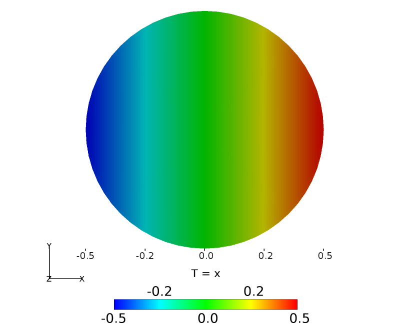
Figure 22 Computational domain and temperature boundary condition for a spherical cavity
The structured O-grid over the spherical wall and on the plane of symmetry is shown in Figure 23. A total of 18564 cells are present within the domain. Over the plane of symmetry, 32 cells are distributed and, over the spherical surface 35 cells are distributed in the radial direction.
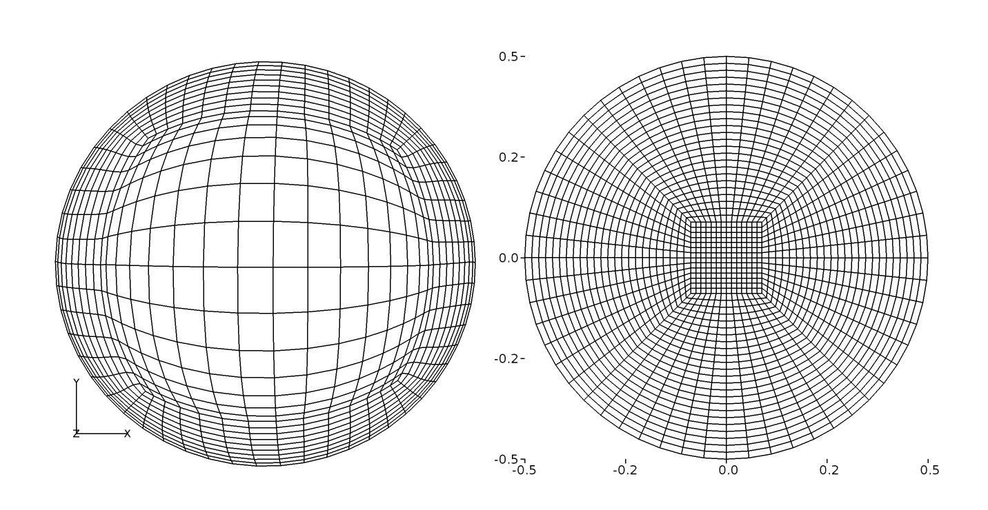
Figure 23 O-grid representation distribution on the wall and on the plane of symmetry
Problem definition
We begin with instructions to set-up the spherical cavity case and the required configuration files that are needed. A full working case is found in the following directory:
/tutorials/heatTransfer/buoyantBoussinesqSimpleSolver/laminar/ACCM_sphericalCavity/
However,the user is free to start the case setup from scratch consistent with the directory stucture discussed below.
Directory Structure
Note
All commands shown here are entered in a terminal window, unless otherwise mentioned
In order to set-up the problem, Caelus requires a time, constant and system sub-directories. Since we will be starting the simulation at time \(t = 0~s\), the time directory would be just 0.
In the 0 sub-directory, few additional files p, p_rgh, alphat, T, and U for pressure, buoyant pressure, turbulent thermal conductivity, temperature and velocity are set respectively. Note that even for a laminar simulation, alphat is required, although a value of 0 would be used. The contents of these files set the dimensions, initialisation and boundary conditions to the case.
The user should be aware that Caelus is case sensitive and therefore the setting up of the directories, files and contents (when applicable) should be identical.
Boundary Conditions and Solver Attributes
Boundary Conditions
The boundary conditions would be set as follows
- Wall
Velocity: Fixed uniform velocity \(u, v, w = 0\)
Pressure: Uniform zero Buoyant Pressure
Temperature: Temperature as a function of \(x\) (\(T = x\))
Turbulent thermal conductivity: Fixed uniform value of 0
- Symmetry Plane
Velocity: Symmetry
Pressure: Symmetry
Temperature: Symmetry
Turbulent thermal conductivity: Symmetry
- Initialisation
Velocity: Fixed uniform velocity \(u, v, w = 0\)
Pressure: Uniform zero Buoyant Pressure
Temperature: Temperature as a function of \(x\) (\(T = x\))
Turbulent thermal conductivity: A value of 0
Note that to specify a temperature as a function of \(x\), swak4Foam library was used and funkySetFields utility was employed. The usage of this would be shown later.
The first quantity to define would be the pressure (\(p\)) and this is done in the file p, which has the following contents.
/*---------------------------------------------------------------------------*\
Caelus 9.04
 Web:      www.caelus-cml.com
\*---------------------------------------------------------------------------*/
FoamFile
{
    version     2.0;
    format      ascii;
    class       volScalarField;
    location    "0";
    object      p;
}
// * * * * * * * * * * * * * * * * * * * * * * * * * * * * * * * * * * * * * //

dimensions      [0 2 -2 0 0 0 0];

internalField   uniform 0;

boundaryField
{
    symm
    {
        type            symmetryPlane;
    }
    wall-1
    {
        type            zeroGradient;
    }
    wall-2
    {
        type            zeroGradient;
    }
}


// ************************************************************************* //
The above file begins with a dictionary named FoamFile containing standard set of keywords such as version, format, location, class and object names. The principle elements follows next
dimensionis used to specify the physical dimensions of the pressure field. Here, pressure is defined in terms of kinematic pressure with the units (\(m^2/s^2\)) written as
[0 2 -2 0 0 0 0]
internalFieldis used to specify the initial conditions. It can be either uniform or non-uniform. Since we have a 0 initial uniform gauge pressure, the entry is
uniform 0;
boundaryFieldis used to specify the boundary conditions. In this case its the boundary conditions for pressure at all the boundary patches.
Similarly, the input data for the buoyant pressure is shown below
/*---------------------------------------------------------------------------*\
Caelus 9.04
 Web:      www.caelus-cml.com
\*---------------------------------------------------------------------------*/
FoamFile
{
    version     2.0;
    format      ascii;
    class       volScalarField;
    location    "0";
    object      p_rgh;
}
// * * * * * * * * * * * * * * * * * * * * * * * * * * * * * * * * * * * * * //

dimensions      [0 2 -2 0 0 0 0];

internalField   uniform 0;

boundaryField
{
    symm
    {
        type            symmetryPlane;
    }
    wall-1
    {
        type            fixedFluxPressure;
        gradient        uniform 0;
        rho             rhok;
        value           uniform 0;
    }
    wall-2
    {
        type            fixedFluxPressure;
        gradient        uniform 0;
        rho             rhok;
        value           uniform 0;
    }
}


// ************************************************************************* //
In the next file, alphat is defined as follows.
/*---------------------------------------------------------------------------*\
Caelus 9.04
 Web:      www.caelus-cml.com
\*---------------------------------------------------------------------------*/
FoamFile
{
    version     2.0;
    format      ascii;
    class       volScalarField;
    location    "0";
    object      alphat;
}
// * * * * * * * * * * * * * * * * * * * * * * * * * * * * * * * * * * * * * //

dimensions      [0 2 -1 0 0 0 0];

internalField   uniform 0;

boundaryField
{
    symm
    {
        type            symmetryPlane;
    }
    wall-1
    {
        type            fixedValue;
        value           uniform 0;
    }
    wall-2
    {
        type            fixedValue;
        value           uniform 0;
    }
}


// ************************************************************************* //
For the temperature, before the funkySetFields expression is used, we need to have the T file with the generic boundary conditions. This is because when funkySetFields is applied, the T file would be overwritten with the profile values.
The final file in this directory is the velocity and the contents are as follows.
/*---------------------------------------------------------------------------*\
Caelus 9.04
 Web:      www.caelus-cml.com
\*---------------------------------------------------------------------------*/
FoamFile
{
    version     2.0;
    format      ascii;
    class       volVectorField;
    location    "0";
    object      U;
}
// * * * * * * * * * * * * * * * * * * * * * * * * * * * * * * * * * * * * * //

dimensions      [0 1 -1 0 0 0 0];

internalField   uniform (0 0 0);

boundaryField
{
    symm
    {
        type            symmetryPlane;
    }
    wall-1
    {
        type            fixedValue;
        value           uniform (0 0 0);
    }
    wall-2
    {
        type            fixedValue;
        value           uniform (0 0 0);
    }
}


// ************************************************************************* //
As noted above, the principle entries for the velocity filed are self explanatory with the typical dimensional units of \(m/s\) ([0 1 -1 0 0 0 0]). The initialisation of the flow is done at \(0~m/s\) which is set using internalField to uniform (0 0 0); which represents three components of velocity.
The boundary conditions (symm, wall-1, wall-2, etc) specified in the above files should be the grid boundary patches (surfaces) that are generated by the grid-generation tool. The user should ensure that their names are identically matched.
Grid file and Physical Properties
The spherical cavity grid is placed in constant/polyMesh sub-directory. Additionally, physical properties are specified in separate files, placed in the constant sub-directory.
The first file is g,wherein the value of acceleration due to gravity is specified. Since we are simulating a buoyancy driven flow, gravity effects should be considered. The contents of g are as follows
/*------------------------------------------------------------------------------*
Caelus 9.04
Web:   www.caelus-cml.com
\*------------------------------------------------------------------------------*/

FoamFile
{
	version     			2.0;
	format      			ascii;
	class      			uniformDimensionedVectorField;
	location    			"constant";
	object      			g;
}
// -------------------------------------------------------------------------------

dimensions      			[0 1 -2 0 0 0 0];

value           			( 0 -9.81 0 );
In the next file transportProperties, details about the transport model for viscosity, Prandtl number, coefficient of thermal expansion are specified. The contents are as follows
/*------------------------------------------------------------------------------*
Caelus 9.04
Web:   www.caelus-cml.com
\*------------------------------------------------------------------------------*/

FoamFile
{
	version				2.0;
	format				ascii;
	class				dictionary;
	location			"constant";
	object				transportProperties;
}

//--------------------------------------------------------------------------------

transportModel				Newtonian;

// Laminar viscosity
nu					nu [0 2 -1 0 0 0 0] 3.4e-4;

// Thermal expansion coefficient
beta					beta [0 0 0 -1 0 0 0] 3.5677e-5;

// Reference temperature
TRef         				TRef [0 0 0 1 0 0 0] 0;

// Laminar Prandtl number
Pr          				Pr [0 0 0 0 0 0 0] 0.7;

// Turbulent Prandtl number
Prt           				Prt [0 0 0 0 0 0 0] 0.7;
Here, Newtonian; keyword is used since the flow is under Newtonian assumption and a kinematic viscosity (\(nu\)) with the units \(m^2/s\) ([0 2 -1 0 0 0 0]) is specified. Similarly, the value of beta, TRef, Pr and Prt are specified. Note that a value of 0.7 is used for laminar Prandtl number.
The type of simulation is specified in turbulenceProperties to laminar using the keyword simulationType as shown below
/*------------------------------------------------------------------------------*
Caelus 9.04
Web:   www.caelus-cml.com
\*------------------------------------------------------------------------------*/

FoamFile
{

	version				2.0;
	format				ascii;
	class				dictionary;
	location			"constant";
	object				turbulenceProperties;
}

//--------------------------------------------------------------------------------

simulationType				laminar;
In addition to this, RASProperties file is required since we specify turbulent thermal conductivity property.
/*-------------------------------------------------------------------------------*
Caelus 9.04
Web:   www.caelus-cml.com
\*------------------------------------------------------------------------------*/

FoamFile
{
	version				2.0;
	format				ascii;
	class				dictionary;
	location			"constant";
	object				RASProperties;
}

//--------------------------------------------------------------------------------

RASModel				laminar;


turbulence				off;

printCoeffs				on;
Controls and Solver Attributes
Here we set-up the necessary files to control the simulation and specifying the solver attributes such as discretization method, linear solver setting, etc and these reside in the system directory.
First, there is the controlDict file with the following information
/*------------------------------------------------------------------------------*
Caelus 9.04
Web:   www.caelus-cml.com
\*------------------------------------------------------------------------------*/
FoamFile
{
    version         2.0;
    format          ascii;
    class           dictionary;
    location        "system";
    object          controlDict;
}
//-------------------------------------------------------------------------------

application         buoyantBoussinesqSimpleSolver;

startFrom           startTime;

startTime           0;

stopAt              endTime;

endTime             2000;

deltaT              1.0;

writeControl        runTime;

writeInterval       10;

purgeWrite          5;

writeFormat         ascii;

writePrecision      12;

writeCompression    uncompressed;

timeFormat          general;

timePrecision       6;

runTimeModifiable   true;


libs (
      "libsimpleSwakFunctionObjects.so"
      "libswakFunctionObjects.so"
      "libgroovyBC.so"
     );
As we will be using funkySetFields, few relevant libraries are needed and they are imported by using the following lines in the controlDict.
libs
(
"libsimpleSwakFunctionObjects.so"
"libswakFunctionObjects.so"
"libgroovyBC.so"
);
The next is the application, buoyantBoussinesqSimpleSolver which is the buoyancy version of the SIMPLE solver that will be used in this simulation. As we begin the simulation at \(t = 0~s\), we need the boundary condition files to be present in the 0 directory, which has been formerly done. The keywords, startTime to startTime is used, where startTime is set to a value 0. The flow is simulated for a total of 2000 iterations and is specified through stopAt and endTime. This is followed by setting the time interval of 10 iterations to save the results via writeControl and writeInterval keywords.
The schemes for finite volume discretization are specified through fvSchemes file with the contents as follows
/*---------------------------------------------------------------------------*
Caelus 9.04
Web:   www.caelus-cml.com
\*---------------------------------------------------------------------------*/
FoamFile
{
    version         2.0;
    format          ascii;
    class           dictionary;
    location        "system";
    object          fvSchemes;
}
//------------------------------------------------------------------------------

ddtSchemes
{
    default         Euler;
}

gradSchemes
{
    default         Gauss linear;
    grad(p)         Gauss linear;
    grad(U)         Gauss linear;
}

divSchemes
{
    default         none;
    div(phi,U)      Gauss linearUpwindBJ grad(U);
    div(phi,T)      Gauss linearUpwindBJ grad(T);
    div((nuEff*dev(T(grad(U))))) Gauss linear;
}

laplacianSchemes
{
    default         none;
    laplacian(rAUf,p_rgh) Gauss linear corrected;
    laplacian(nu,U) Gauss linear corrected;
    laplacian(nuEff,U) Gauss linear corrected;
    laplacian(alphaEff,T) Gauss linear corrected;
    laplacian(p_rgh) Gauss linear corrected;
    laplacian(kappaEff,T) Gauss linear corrected;
    laplacian((1|A(U)),p) Gauss linear corrected;
    laplacian((1|A(U)),p_rgh) Gauss linear corrected;
}

interpolationSchemes
{
    default         linear;
    interpolate(HbyA) linear;
}

snGradschemes
{
    default         corrected;
}
In the above file, the discretization schemes are set for time-derivative, gradient, divergence and Laplacian terms.
The final file is the fvSolution, where linear solver settings are provided and is as given below
/*---------------------------------------------------------------------------*
Caelus 9.04
Web:   www.caelus-cml.com
\*---------------------------------------------------------------------------*/
FoamFile
{
    version     2.0;
    format      ascii;
    class       dictionary;
    location    "system";
    object      fvSolution;
}
//------------------------------------------------------------------------------

solvers
{
    p_rgh
    {
        solver           GAMG;
        tolerance        1e-8;
        relTol           0.01;
        smoother         SSGS;
        cacheAgglomeration true;
        nCellsInCoarsestLevel 10;
        agglomerator     algebraicPair;
        mergeLevels      1;
    }

    "(U|T)"
    {
        solver          PBiCGStab;
        preconditioner  USGS;
        tolerance       1e-8;
        relTol          0.01;
    }
}

SIMPLE
{
    nNonOrthogonalCorrectors 0;
    pRefCell        0;
    pRefValue       0;

    residualControl
    {
        p_rgh           1e-4;
        T               1e-4;

        // possibly check turbulence fields
    }
}

relaxationFactors
{
    fields
    {
        p_rgh           0.3;
    }
    equations
    {
        U               0.7;
        T               0.7;
    }
}


// ************************************************************************* //
The above file details the different linear solvers that are used to solve for buoyant pressure and velocity fields. Further, nNonOrthogonalCorrectors is set to 2; since there is some degree of non-orthogonality present in the grid.
With these, the set-up of the relevant directories and files are completed. Let us view the directory structure to ensure all are present. The tree should be identical to the one shown below
tree
.
├── 0
│   ├── alphat
│   ├── p
│   ├── p_rgh
│   ├── T
│   └── U
├── constant
│   ├── polyMesh
│   │   ├── boundary
│   │   ├── faces
│   │   ├── neighbour
│   │   ├── owner
│   │   └── points
│   ├── RASProperties
│   ├── transportProperties
│   └── turbulenceProperties
└── system
    ├── controlDict
    ├── fvSchemes
    └── fvSolution
Execution of the solver
Before the solver can be executed, we have to apply the temperature profile as noted earlier. This step can be performed as follows
funkySetFields -field T -expression "pos().x" -time 0 -keepPatches -valuePatches "wall-1 wall-2"
The above expression re-writes the T file with the appropriate values of temperature as a function of distance \(x\). Following this, the solver can be executed and it involves few different steps. The first of which is to renumber the grid or mesh followed by checking the mesh quality. Renumbering reduces the matrix bandwidth while quality check shows the mesh statistics. These can be performed as follows
caelus run -- renumberMesh -overwrite
caelus run -- checkMesh
During the process of renumbering, grid-cell bandwidth information before and after renumberMesh is shown and the user can take a note of this. The mesh statistics are as shown below after invoking checkMesh
/*---------------------------------------------------------------------------*\
 Caelus 8.04
 Web:      www.caelus-cml.com
\*---------------------------------------------------------------------------*/

Checking geometry...
    Overall domain bounding box (-0.5 -0.5 0) (0.5 0.5 0.5)
    Mesh (non-empty, non-wedge) directions (1 1 1)
    Mesh (non-empty) directions (1 1 1)
    Boundary openness (2.69541574409e-17 -1.48776322194e-17 -2.09950188835e-16) OK.
    Max cell openness = 2.71077471766e-16 OK.
    Max aspect ratio = 5.13298999541 OK.
    Minimum face area = 7.26421673269e-05. Maximum face area = 0.0145134277912.  Face area magnitudes OK.
    Min volume = 8.32359098625e-07. Max volume = 0.000256180182954.  Total volume = 0.259143943239.  Cell volumes OK.
    Mesh non-orthogonality Max: 64.2010673845 average: 15.1363376112
    Non-orthogonality check OK.
    Face pyramids OK.
    Mesh skewness Max: 0.60153646289 average: 0.0467687348165 OK.
    Coupled point location match (average 0) OK.

Mesh OK.

End
The above information gives a maximum mesh non-orthogonality angle of 64.2 and therefore non-orthogonal corrections are needed for the solver. In the next step, we will execute the solver and monitor the progress of the simulation. The solver should be executed from the top level directory using,
caelus run -l my-spherical-cavity.log buoyantBoussinesqSimpleSolver
The progress of the simulation is written to the log file my-spherical-cavity.log, which can be monitored to view the convergence history. In a separate terminal window use
caelus logs -w my-spherical-cavity.log
The plot indicates the convergence history for pressure with respect to time and a similar plot is shown in Figure 24. The convergence of other properties can also be found by using the above command.
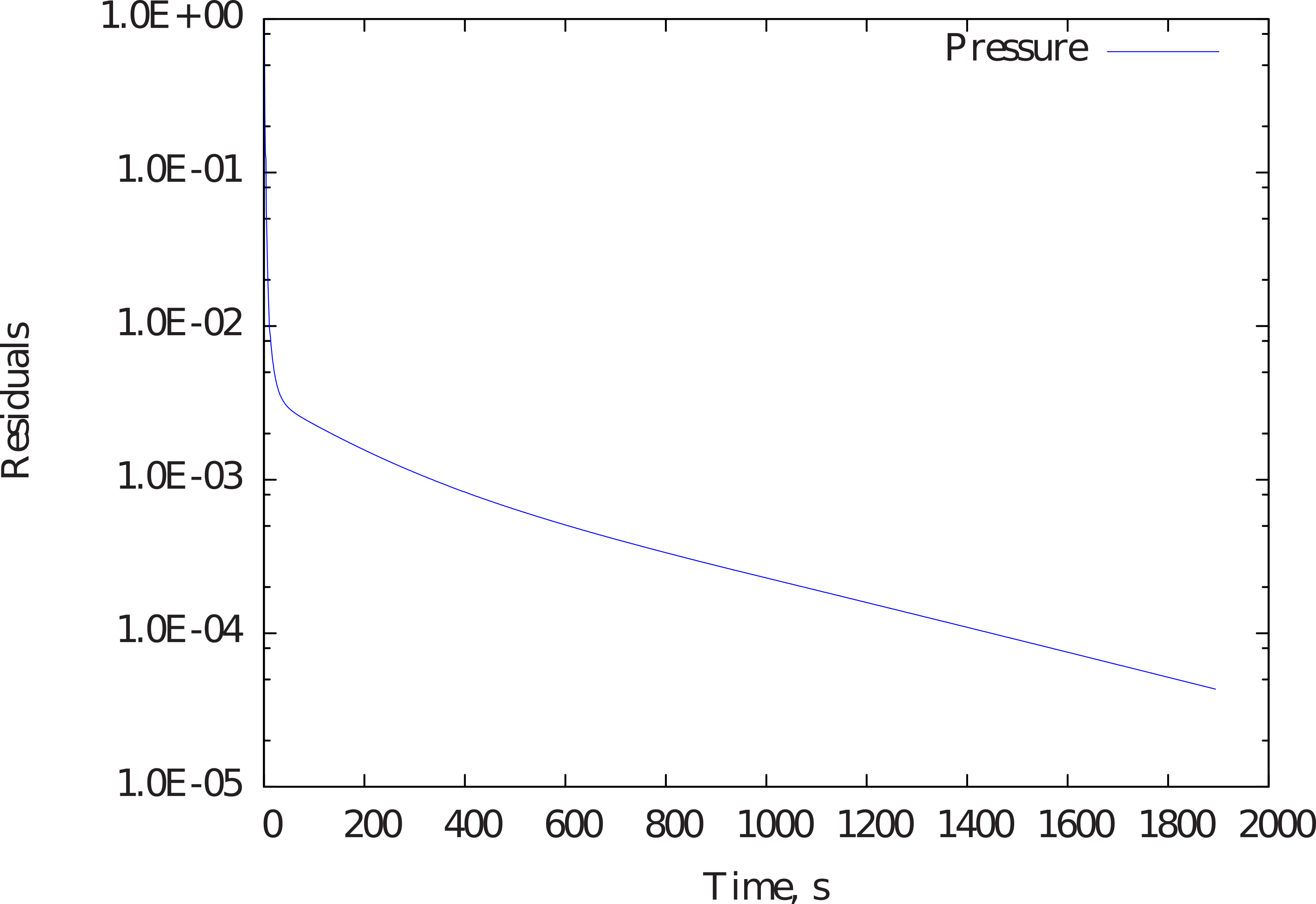
Figure 24 Convergence of pressure with respect to time
Results
Here, the solution obtained at steady state is shown and is compared with the analytical solution. In Figure 25, the comparison of temperature isotherms is presented. The analytical solution is a first order approximation. A close agreement between the two can be observed.
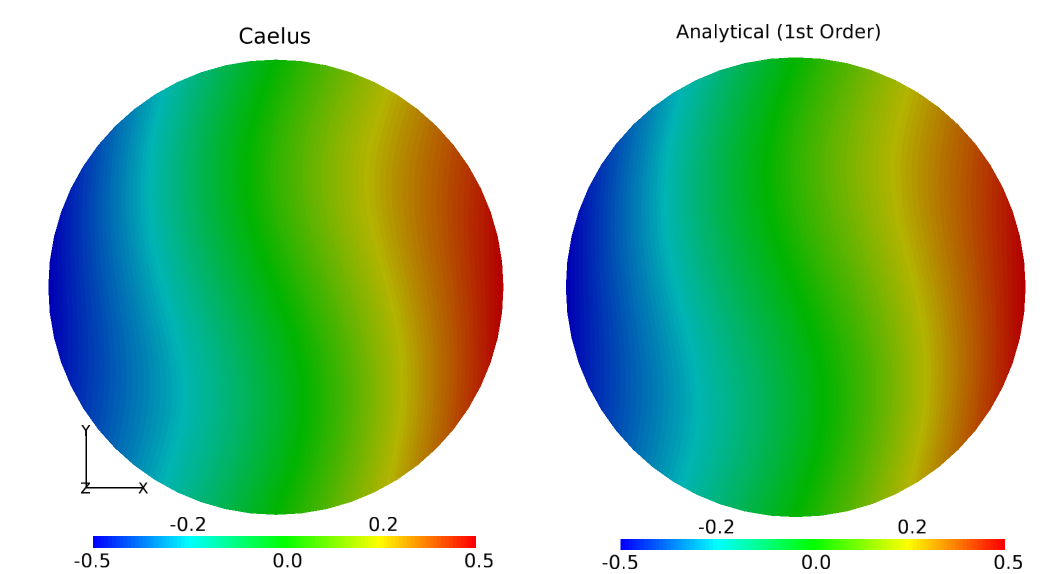
Figure 25 Comparison of temperature isotherms between computational and analytical solutions.