Validation: Incompressible Laminar Flows
This section details the validation work carried out in Caelus 9.04 for several conditions ranging from attached to separated flows. Both transient and steady state conditions have been considered under laminar and turbulent flows for relevant cases.
Flat-plate
Laminar, incompressible flow over a two-dimensional Sharp-Leading Edge flat-plate
Nomenclature
Symbol |
Definition |
Units (SI) |
|---|---|---|
\(c_f\) |
Skin friction coefficient |
Non-dimensional |
\(e\) (subscript) |
Boundary layer edge conditions |
|
\(L\) |
Length of the plate |
\(m\) |
\(p\) |
Kinematic pressure |
\(Pa/\rho~(m^2/s^2)\) |
\(Re\) |
Reynolds number |
Non-dimensional |
\(T\) |
Temperature |
\(K\) |
\(u\) |
Local velocity in x-direction |
\(m/s\) |
\(U\) |
Freestream velocity in x-direction |
\(m/s\) |
\(x\) |
Distance in x-direction |
\(m\) |
\(y\) |
Distance in y-direction |
\(m\) |
\(\nu\) |
Kinematic viscosity |
\(m^2/s\) |
\(\eta\) |
Blasius parameter |
Non-dimensional |
Introduction
In this validation case, steady, incompressible, laminar flow over a two-dimensional sharp-leading edge flat-plate at zero angle of incidence is investigated. The flow generates a laminar boundary layer and the computational results are compared with the Blasius solution for the incompressible flow. Validation of the flow over a flat-plate forms the basis of these validation efforts as it is perhaps the most well understood configuration for CFD code-validation.
Blasius, in his work [6] obtained the solution to the Boundary Layer Equations using a transformation technique. Here, equations of continuity and momentum in two-dimensional form are converted into a single ordinary differential equation (ODE). The solution to this ODE can be numerically obtained and is regarded as the exact solution to the boundary layer equations. It is only valid for steady, incompressible, laminar flow over a flat-plate. One of the highlights of Blasius solution is the analytical expression for the skin friction coefficient (\(c_f\)) distribution along the flat-plate given by
where \(Re_{x}\) is the local Reynolds number defined as
\(U\) is the freestream velocity, \(x\) is the distance starting from the leading edge and \(\nu\) is the kinematic viscosity.
Problem definition
This exercise is based on the validation work carried out by the NASA NPARC alliance for a flow over a flat-plate using the same conditions in the incompressible limit. A schematic of the geometric configuration is shown in Figure 52.

Figure 52 Schematic representation of the flat plate
The length of the plate is L = 0.3048 m wherein, x = 0 is the leading edge, the Reynolds number of the flow based on the length of the plate is 200,000 and U is the velocity in the x-direction. Assuming the inlet flow is at a temperature of 300 K, the kinematic viscosity can be determined from dynamic viscosity and density of the fluid. The value is given in the table below. The value of dynamic viscosity is obtained from the Sutherland viscosity formulation. Using the Reynolds number, plate length and kinematic viscosity, the freestream velocity evaluates to U = 10.4306 m/s. The following table summarises the freestream conditions used:
Fluid |
\(Re\) |
\(U~(m/s)\) |
\(p~(m^2/s^2)\) |
\(T~(K)\) |
\(\nu~(m^2/s)\) |
|---|---|---|---|---|---|
Air |
200,000 |
10.43064 |
\((0)\) Gauge |
300 |
\(1.58963\times10^{-5}\) |
As we have assumed the flow incompressible, the density (\(\rho\)) remains constant. In addition, since the fluid temperature is not considered, the viscosity remains constant. For incompressible flows, the kinematic forms of pressure and viscosity are always used in Caelus.
Computational Domain and Boundary Conditions
The computational domain is a rectangular block encompassing the flat-plate. Figure 53 shows the details of the boundaries used in two-dimensions (\(x-y\) plane). As indicated in blue, the region of interest extends between \(0\leq x \leq 0.3048~m\) and has a no-slip boundary condition. Upstream of the leading edge, a slip boundary is used to simulate freestream uniform flow approaching the flat-plate. However, downstream of the plate, there is additional no-slip wall a further three plate lengths (highlighted in green). This ensures that the boundary layer in the vicinity of the trailing edge is not influenced by the outlet boundary. Since the flow is subsonic, disturbances cause the pressure to propagate both upstream and downstream. Therefore, placement of the inlet and outlet boundaries were chosen to have minimal effect on the solution. The inlet boundary as shown in the figure below is placed at start of the slip-wall (\(x = -0.06~m\)) and the outlet at the end of the second no-slip wall (\(x = 1.2192~m\)). Both inlet and outlet boundaries are between \(0\leq y \leq 0.15~m\). A slip-wall condition is used for the entire top boundary.

Figure 53 Flat plate computational domain
Boundary Conditions and Initialisation
The following are the boundary condition details used for the computational domain:
- Inlet
Velocity: Fixed uniform velocity \(u = 10.4306~m/s\) in \(x\) direction
Pressure: Zero gradient
- Slip wall
Velocity: Slip
Pressure: Slip
- No-slip wall
Velocity: Fixed uniform velocity \(u, v, w = 0\)
Pressure: Zero gradient
- Outlet
Velocity: Zero gradient velocity
Pressure: Fixed uniform gauge pressure \(p = 0\)
- Initialisation
Velocity: Fixed uniform velocity \(u = 10.4306~m/s\) in \(x\) direction
Pressure: Zero Gauge pressure
Computational Grid
A 2D structured grid was generated using Pointwise in the \(x-y\) plane. Since Caelus is a 3D computational framework, it necessitates the grid to also be 3D. Therefore, a 3D grid was obtained using Pointwise by extruding the 2D grid in the positive \(z\) direction by one cell. The final 3D grid was then exported to the Caelus format (polyMesh). The two \(x-y\) planes obtained as a result of grid extrusion need boundary conditions to be specified. As the flow over a flat-plate is generally 2D, we do not need to solve the flow in the third dimension. This is achieved in Caelus by specifying empty boundary condition for each plane. Although, no flow is computed in the \(z\) direction, a velocity of \(w = 0\) has to be specified for the velocity boundary condition as indicated above.
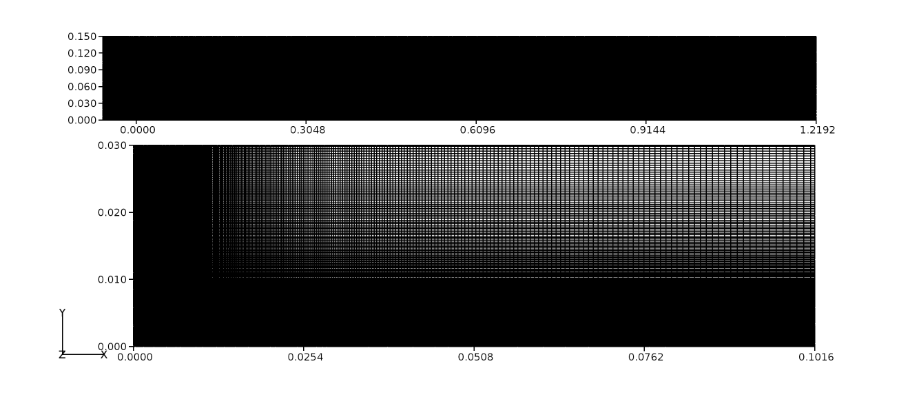
Figure 54 Structured grid for a flat plate domain
Figure 54 shows the 2D grid in the \(x-y\) plane. As can be seen, the grid is refined perpendicular to the wall in order to capture resolve the viscous effects. To ensure that the gradients in boundary layer are well resolved, about 50 grid nodes are placed between the wall and the boundary layer edge. Grid refinement is also added at the leading edge so that the growth of the boundary layer is also well resolved. In this particular case, 400 cells were used in the stream-wise (\(x\)) direction (\(x \leq 0 \leq 0.3048~m\)) and 600 in the wall normal (\(y\)) direction. For no-slip wall beyond \(x > 0.3048\), a similar distribution is used.
Results and Discussion
A time-dependent solution to the two-dimensional flat-plate was obtained using Caelus 9.04. The SLIM transient solver was used here and the flow was simulated sufficiently long (several plate length flow times) such that steady flow was established. For the discretization of time-dependent terms, the first-order Euler scheme was used. A Gauss linear discretization was used for the pressure and velocity gradients. A linear upwind discretization was for the divergence of velocity and mass flux. A linear corrected scheme was used for Laplacian discretization while cell-to-face centre interpolation used linear interpolation.
In Figure 55, the skin-friction distribution along the flat-plate obtained from the CFD simulation is compared with that of the Blasius analytical solution. Here, the distance \(x\) is normalised with the length of the plate (\(L\)). Excellent agreement is observed along the entire length of the flat-plate.
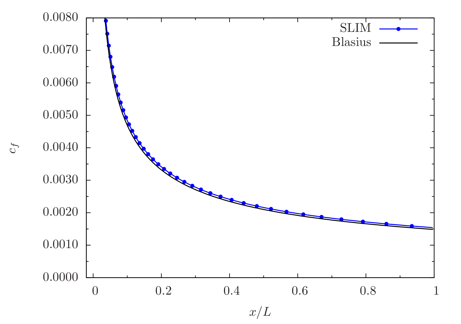
Figure 55 Skin-friction comparison between SLIM and Blasius solutions
At the exit plane of the flat-plate at \(x = 0.3048~m\), velocity data was extracted across the boundary layer and compared with the Blasius analytical solution. This is shown in Figure 56 where the velocity profile is plotted using similarity variables from the Blasius solution. Here, \(\eta\) is the non-dimensional distance from the wall to the boundary layer edge and \(U_e\) is the velocity at the boundary layer edge. Similar to skin-friction, the velocity profile also exhibits excellent agreement with the Blasius solution.
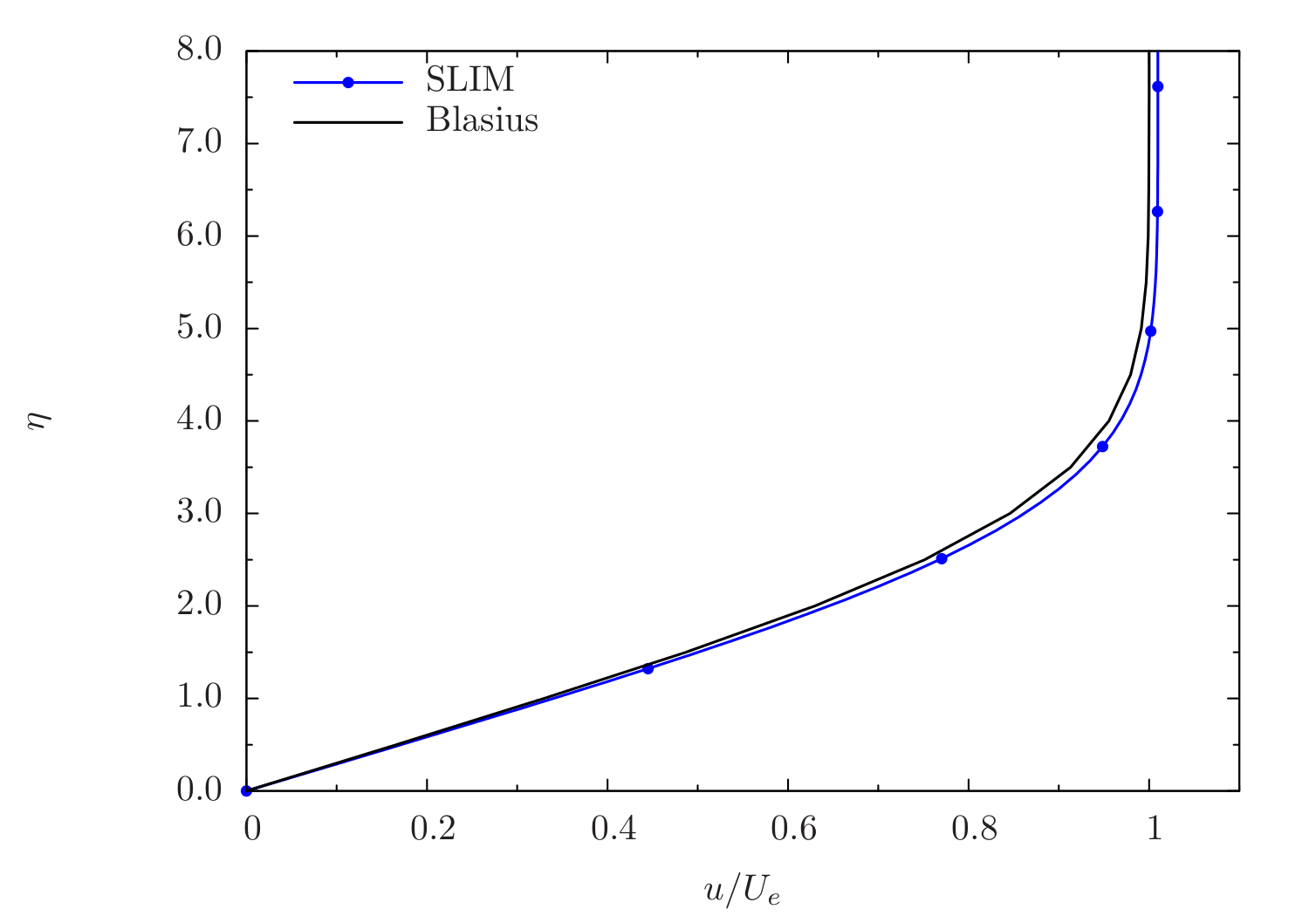
Figure 56 Non-dimensional velocity profile comparison between SLIM and Blasius solutions
Conclusions
The steady, incompressible, laminar flow over a two-dimensional flat-plate was simulated using Caelus 9.04 utilising the SLIM solver. The results were validated against the Blasius analytical solutions resulting in excellent agreement.
Tee Junction
Laminar, incompressible flow in a 90 degree tee junction
Nomenclature
Symbol |
Definition |
Units (SI) |
|---|---|---|
\(L\) |
Length of the branch |
\(m\) |
\(p\) |
Kinematic pressure |
\(Pa/\rho~(m^2/s^2)\) |
\(Re_w\) |
Reynolds number based on width |
Non-dimensional |
\(V\) |
Freestream velocity in y-direction |
\(m/s\) |
\(W\) |
Width of the branch |
\(m\) |
\(x\) |
Distance in x-direction |
\(m\) |
\(y\) |
Distance in y-direction |
\(m\) |
\(\nu\) |
Kinematic viscosity |
\(m^2/s\) |
Introduction
In this validation case, laminar, incompressible flow through a two-dimensional \(90^\circ\) tee junction was investigated. Due to the presence of the side branch, the flow separates and forms a recirculating region. The recirculating regions influences the mass flow through the main and side branches. The numerically computed mass-flow ratio was calculated and compared with experiment.
A comprehensive study of flow through planar branches has been carried out by Hayes et al. [12] due to its prevelance in the bio-mechanical industry. Of which, the \(90^\circ\) right-angled tee junction is considered here for the purpose of validation.
Problem definition
The following figure shows the schematic of the tee-junction. Here, L = 3.0 m, W = 1.0 m respectively, the Reynolds number based on the width is 300, and V is the velocity in the y-direction. For simplicity, we have assumed the velocity, V = 1 m/s. Using these values the resulting kinematic viscosity was 0.00333 \(m^2/s\).
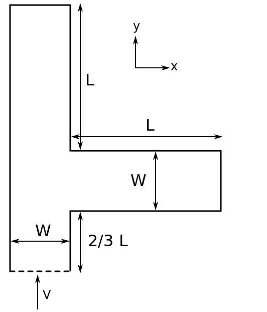
Figure 57 Tee-junction Schematic
The summary of the flow properties and geometric details are given in the following table.
\(Re_w\) |
\(L\) |
\(W\) |
\(V~(m/s)\) |
\(p~(m^2/s^2)\) |
\(\nu~(m^2/s)\) |
|---|---|---|---|---|---|
300 |
3.0 |
1.0 |
1.0 |
\((0)\) Gauge |
0.00333 |
As we have assumed the flow incompressible, the density (\(\rho\)) remains constant. In addition, since the fluid temperature is not considered, the viscosity remains constant. For incompressible flows, the kinematic forms of pressure and viscosity are always used in Caelus.
Computational Domain and Boundary Conditions
Since this is an internal flow problem, the computational domain is contained within tee-junction geometry. The details are shown in Figure 58. As indicated, all tee-junction walls have a no-slip boundary condition which has been highlighted in blue. At the inlet, a fully developed laminar flow parabolic profile is applied, otherwise a much longer main branch would be required for the flow to develop. The domain has two outlets, one at the end of the main channel and the other at the end of side branch. Note the exit pressures at the two outlets are equal.

Figure 58 Computational domain representing tee-junction
Boundary Conditions and Initialisation
The following are the boundary condition details used for the computational domain:
- Inlet
Velocity: Parabolic velocity profile; centerline velocity of \(v = 1.0~m/s\) in \(y\) direction
Pressure: Zero gradient
- No-slip wall
Velocity: Fixed uniform velocity \(u, v, w = 0\)
Pressure: Zero gradient
- Outlet-1
Velocity: Zero gradient velocity
Pressure: Fixed uniform gauge pressure \(p = 0\)
- Outlet-2
Velocity: Zero gradient velocity
Pressure: Fixed uniform gauge pressure \(p = 0\)
- Initialisation
Velocity: Fixed uniform velocity \(u, v, w = 0\)
Pressure: Zero Gauge pressure
Computational Grid
The 2D structured grid is shown in Figure 59. Since Caelus is a 3D computational framework, it necessitates the grid to also be 3D. Therefore, a 3D grid was obtained by extruding the 2D grid in the positive \(z\) direction by one cell. The final 3D grid was then exported to the Caelus format (polyMesh). The two \(x-y\) planes obtained as a result of grid extrusion need boundary conditions to be specified. As the flow over a flat-plate is generally 2D, we do not need to solve the flow in the third dimension. This is achieved in Caelus by specifying empty boundary condition for each plane. Although, no flow is computed in the \(z\) direction, a velocity of \(w = 0\) has to be specified for the velocity boundary condition as indicated above.
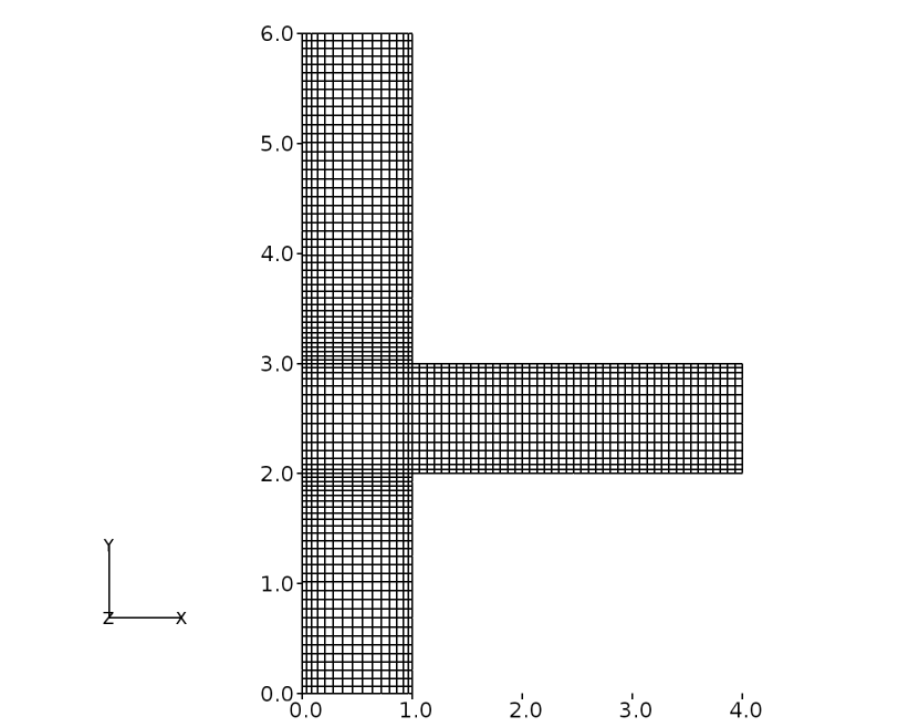
Figure 59 Structured grid for tee-junction domain
A total of 2025 cells comprise the tee-junction of which, 90 cells are distributed along the height of the main channel, and 45 along the length of the side branch. The distribution is such that a dimensional length of \(L = 1~m\) has a total of 45 cells, giving a distribution of \((2/3)*45 = 30\) cells for the \((2/3) L\) segment of the main channel. The width, \(W\), consists of 15 cells.
Results and Discussion
A time-dependent solution to the two-dimensional flat-plate was obtained using Caelus 9.04. The SLIM transient solver was used here and the flow was simulated sufficiently long such that steady separated flow was established. To ensure this, shear-stress distribution was monitored on the lower wall of the side branch. The simulation was stopped once the separation and reattachment locations no longer varied with time.
Mass flow was calculated at the inlet and at the main outlet (outlet-1) and the mass-flow ratio was subsequently calculated. The below table compares the SLIM result with the experimental value. As can be noted, the agreement between the two is excellent.
Experimental |
SLIM |
Percentage Difference |
|
|---|---|---|---|
Flow Split |
\(0.887\) |
\(0.886\) |
\(0.112~\%\) |
Conclusions
The steady, incompressible, two-dimensional laminar flow in a right-angled \(90^\circ\) tee-junction was simulated using Caelus 9.04 with the SLIM solver and validated against experimental data resulting in excellent agreement.
Circular Cylinder
Laminar, incompressible flow over a circular cylinder
Nomenclature
Symbol |
Definition |
Units (SI) |
|---|---|---|
\(D\) |
Diameter of the cylinder |
\(m\) |
\(f\) |
Frequency |
\(hz\) |
\(p\) |
Kinematic pressure |
\(Pa/\rho~(m^2/s^2)\) |
\(Re_D\) |
Reynolds number based on diameter |
Non-dimensional |
\(St\) |
Strouhal number |
Non-dimensional |
\(U\) |
Freestream velocity in x-direction |
\(m/s\) |
\(x\) |
Distance in x-direction |
\(m\) |
\(y\) |
Distance in y-direction |
\(m\) |
\(\nu\) |
Kinematic viscosity |
\(m^2/s\) |
In this validation study, laminar incompressible flow over a 2D circular cylinder is investigated at a Reynolds number of 100. This classical configuration represents flow over a bluff body dominated by a wake region. For flows having a low Reynolds number (\(40 \leq Re_D \leq 150\)), periodic vortex shedding occurs in the wake. The phenomenon of vortex shedding behind bluff bodies is referred to as the Karman Vortex Street [2] and provides an transient case for CFD code validation.
In his work, Roshko [2] experimentally studied wake development behind two-dimensional circular cylinders from Reynolds number ranging from 40 to 10000. For Reynolds numbers of 40 to 150, the so called the stable range [Roshko1954], regular vortex streets are formed with no evidence of turbulence motion in the wake. Therefore, at a Reynolds number of 100, the vortex shedding exhibits smooth, coherent structures making it ideally suited for validating laminar CFD calculations. The frequency associated with the oscillations of the vortex streets can be characterized by the Strouhal Number (\(St\)). The Strouhal Number is a non-dimensional number defined as
where, \(f\) is the frequency of oscillations of vortex shedding, \(D\) is the diameter of the cylinder and \(U\) is the freestream velocity of the flow. Experimentally [Roshko1954], it has been determined that for a Reynolds number based on the diameter of the cylinder of 100, the Strouhal number \(St \approx 0.16 - 0.17\). One of the main objectives in this study was to compare the \(St\) for the CFD calculation to the experimental data of Roshko [Roshko1954]. Provided the cylinder has a sufficient span length, the flow characteristics can be assumed to be two-dimensional as the experiments suggest.
Problem Definition
Figure 60 shows the schematic of the two-dimensional circular cylinder. Here, the diameter D = 2 m and is the characteristic length for the Reynolds number, which is 100. For simplicity, the freestream velocity was taken to be U = 1 m/s in the x direction. Using these values the kinematic viscosity was calculated to be 0.02 \(m^2/s\).

Figure 60 Schematic representation of a circular cylinder
In the table below, a summary of the freestream conditions are provided
\(Re_D\) |
\(D\) |
\(U~(m/s)\) |
\(p~(m^2/s^2)\) |
\(\nu~(m^2/s)\) |
|---|---|---|---|---|
100 |
2.0 |
1.0 |
\((0)\) Gauge |
0.02 |
Here, the flow is assumed to be incompressible and therefore the density is constant. Further, no temperature is evaluated in this calculation and hence the viscosity also remains constant. For incompressible flows, the kinematic forms of pressure and viscosity are always used in Caelus.
Computational Domain and Boundary Conditions
A rectangular computational domain in the \(x-y\) plane was constructed surrounding the circular cylinder as shown in Figure 61. A full cylinder must be used due to the oscillatory nature of the shed vortices. Rhe domain extends by 5 diameters of cylinder and 20 diameters downstream. Since the flow here is viscous dominated, sufficient downstream length is required to capture the vortex separation from the surface of the cylinder and the subsequently shedding in the wake. In the \(y\) direction, the domain extends 5 diameters on either side. From the figure, multiple inlet boundaries to this domain can be seen, one at the upstream boundary and the other two for the top and bottom boundaries. This type of configuration is needed to appropriately model the inflow, similar to an undisturbed flow in an experimental set-up. It is noted that for top and bottom boundaries, the flow is in the \(x\) direction. The outlet is located at the downstream boundary. The cylindrical wall is a no-slip boundary condition.

Figure 61 Computational domain of a circular cylinder
Boundary Conditions and Initialisation
Following are the details of the boundary conditions used:
- Inlet-1
Velocity: Fixed uniform velocity \(u = 1.0~m/s\) in \(x\) direction
Pressure: Zero gradient
- Inlet-2
Velocity: Fixed uniform velocity \(u = 1.0~m/s\) in \(x\) direction
Pressure; Zero gradient
- No-slip wall
Velocity: Fixed uniform velocity \(u, v, w = 0\)
Pressure: Zero gradient
- Outlet
Velocity: Zero gradient velocity
Pressure: Fixed uniform gauge pressure \(p = 0\)
- Initialisation
Velocity: Fixed uniform velocity \(u = 1.0~m/s\) in \(x\) direction
Pressure: Zero Gauge pressure
Computational Grid
The computational grid in 2D was generated using Pointwise in the \(x-y\) plane. Since Caelus is a 3D computational framework, it necessitates the grid to also be 3D. Therefore, a 3D grid was obtained using Pointwise by extruding the 2D grid in the positive \(z\) direction by one cell. The final 3D grid was then exported to the Caelus format (polyMesh). The two \(x-y\) planes obtained as a result of grid extrusion need boundary conditions to be specified. As the flow over a flat-plate is generally 2D, we do not need to solve the flow in the third dimension. This is achieved in Caelus by specifying empty boundary condition for each plane. Although, no flow is computed in the \(z\) direction, a velocity of \(w = 0\) has to be specified for the velocity boundary condition as indicated above.
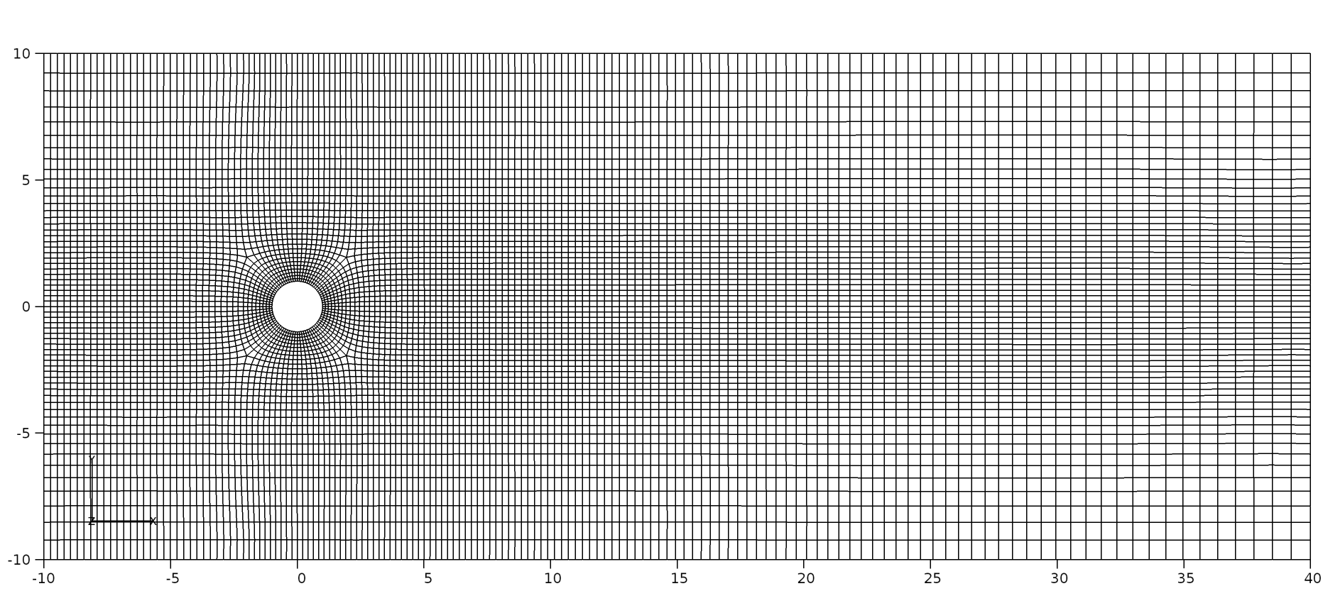
Figure 62 O-grid around the cylinder and structured gird representation
The 2D domain consisted of 9260 cells. An O-grid topology was constructed around the cylinder (see the right figure) with 10 cells in the radial direction and 84 cells in the circumferential direction. 31 cells were used upstream of the O-grid, in the \(x\) direction while 100 cells were used downstream. The region of interest is about 10 diameters downstream, where the grids are refined. In the \(y\) direction, 21 cells were used above and below the O-grid region.
Results and Discussion
A time-dependent simulation was carried out using the Caelus 9.04 with the SLIM solver. To capture the transient start-up process, the calculation was started from time t = 0 s and was simulated up to t = 360 s, while lift and drag forces over the cylindrical surface were monitored at a frequency of 2 Hz. It was found that the on-set of vortex shedding occurred after about t = 90 s which was then followed by a steady shedding process. A Fast Fourier transformation (FFT) was carried out on the lift force data and the peak frequency of vortex shedding occurred at \(f = 0.0888\) Hz. Based on this value, it takes about 7.8 cycles for the shedding to start.
Using the peak frequency value of \(f = 0.0888\) Hz, \(St\) was evaluated. The table below compares the computed value from SLIM with that of the experiment. The agreement is good given that experimental uncertainty can be relatively high at low Reynolds numbers.
Frequency (Hz) |
Strouhal Number |
|
|---|---|---|
Experimental |
0.0835 |
\(0.167\) |
SLIM |
0.0888 |
\(0.177\) |
Conclusions
The transiet, incompressible, two-dimensional flow over a circular cylinder was simulated using Caelus 9.04 to estimate the peak frequency of vortex shedding. The value was compared to well known experimental data resulting in good agreement.
Triangular Cavity
Laminar, incompressible flow inside a lid driven Triangular Cavity
Nomenclature
Symbol |
Definition |
Units (SI) |
|---|---|---|
\(D\) |
Depth of the cavity |
\(m\) |
\(p\) |
Kinematic pressure |
\(Pa/\rho~(m^2/s^2)\) |
\(Re_D\) |
Reynolds number based on depth |
Non-dimensional |
\(U\) |
Freestream velocity in x-direction |
\(m/s\) |
\(W\) |
Width |
\(m\) |
\(x\) |
Distance in x-direction |
\(m\) |
\(y\) |
Distance in y-direction |
\(m\) |
\(\nu\) |
Kinematic viscosity |
\(m^2/s\) |
This validation study concerns the laminar, incompressible flow inside a lid driven triangular cavity. Here, the top wall of the cavity moves at a constant velocity initiating a recirculating motion within the cavity. Due to the viscous nature of the flow, a boundary layer develops in the direction of the moving lid, while flow reversal occurs due to the recirculating flow. The flow feature of interest is the velocity distribution along the centre-line of the cavity.
Benchmark experiments on this configuration has been reported in Jyotsna and Venka [11] for a Reynolds number of 800. The main objective of this validation case was to compare the \(x\) velocity distribution against experimental data.
Problem Definition
A schematic of the triangular cavity is presented in Figure 63 where depth of the cavity D = 4 m and the width W = 2 m. The Reynolds number based on the cavity depth is 800 and the wall velocity is U = 2 m/s. Using the Reynolds number, U, and D, kinematic viscosity was calculated to be 0.01 \(m^2/s\).

Figure 63 Schematic showing the Triangular Cavity
The table below summaries the flow properties
\(Re_D\) |
\(D~(m)\) |
\(W~(m)\) |
\(U~(m/s)\) |
\(p~(m^2/s^2)\) |
\(\nu~(m^2/s)\) |
|---|---|---|---|---|---|
800 |
4.0 |
2.0 |
2.0 |
\((0)\) Gauge |
\(0.01\) |
The flow in this case is assumed to be incompressible and hence the density remained constant throughout. Further, the temperature field is not accounted into the calculation, and therefore the viscosity of the flow can also remain constant. Since viscosity is constant, it becomes more convenient to specify it as kinematic viscosity. It should be noted that in Caelus for incompressible flows, both pressure and viscosity are always specified as kinematic.
Computational Domain and Boundary Conditions
The computational domain is the triangular cavity shown in Figure 64. Highlighted in blue, the side walls of the cavity have a no-slip boundary condition while the top wall, highlighted in green, has a uniform velocity in the \(x\) direction.

Figure 64 Computational domain of a Triangular Cavity
Boundary Conditions and Initialisation
- Moving wall
Velocity: Fixed uniform velocity \(u = 2.0~m/s\) in \(x\) direction
Pressure: Zero gradient
- No-slip wall
Velocity: Fixed uniform velocity \(u, v, w = 0\)
Pressure: Zero gradient
- Initialisation
Velocity: Fixed uniform velocity \(u, v, w = 0\)
Pressure: Zero Gauge pressure
Computational Grid
The 2D grid in \(x-y\) plane is shown in Figure 65. A hybrid grid is employed for this case with a total of 5538 cells. Up to a depth of D = 1.35 m a structured grid is used while below that value an unstructured triangular grid is used. An unstructured grid is used in the bottom portion because it resulted in lower skewness in this vicinity. For the structured region, 40 cells are distributed across the width of the cavity and 40 along the depth. The cavity walls in the unstructured region have 100 cells along each. The interface of the two regions is node matched and has 40 cells across the width. The grid close to the cavity lid was refined to better capture the shear layer.
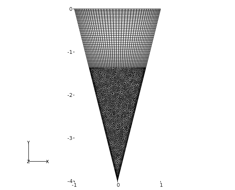
Figure 65 Hybrid grid for a Triangular Cavity
The flow characteristics in the cavity can be assumed to be two dimensional and here it has been solved with the same assumption. Since Caelus is a 3D computational framework, it necessitates the grid to also be 3D. Therefore, a 3D grid was obtained using Pointwise by extruding the 2D grid in the positive \(z\) direction by one cell. The final 3D grid was then exported to the Caelus format (polyMesh). The two \(x-y\) planes obtained as a result of grid extrusion need boundary conditions to be specified. As the flow over a flat-plate is generally 2D, we do not need to solve the flow in the third dimension. This is achieved in Caelus by specifying empty boundary condition for each plane. Although, no flow is computed in the \(z\) direction, a velocity of \(w = 0\) has to be specified for the velocity boundary condition as indicated above.
Results and Discussion
A steady solution to the cavity was obtained using Caelus 9.04 with the SLIM solver. While a time-dependent approach was used, the solution was simulated sufficiently long so that steady flow was achieved. To determine when this occured the velocity distribution along the cavity centre-line was monitored with respect to time. The simulations was stopped when no appreciable changes were observed.
In Figure 66, the \(x\) velocity distribution along the cavity centre-line is compared with that of the benchmark experimental data. The \(y\) distance is normalised with the cavity depth (\(D\)) which gives \(y/d = 0\) at the cavity lid and \(y/d = -1\) at the bottom vertex. Similarly, the \(u\) velocity is normalised with the velocity of the cavity lid (\(u_L\)).
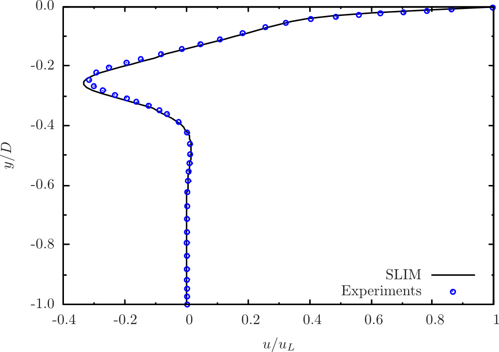
Figure 66 Comparison of experimental and computational \(x\) velocity distribution along the cavity’s centre-line
As seen in Figure 66 above, the comparison the experiment is excellent.
Conclusions
A steady, incompressible flow past a two-dimensional triangular cavity was simulated using Caelus 9.04 on a hybrid grid. The velocity distribution along the centre-line of the cavity was compared with the benchmark experimental data, it was found that the SLIM results compared very favorably.
Spherical Cavity
Natural Convection in a Spherical Cavity
Nomenclature
Symbol |
Definition |
Units (SI) |
|---|---|---|
\(C_p\) |
Specific heat at constant pressure |
\(J/kg \cdot K\) |
\(D\) |
Diameter of the sphere |
\(m\) |
\(g\) |
Gravitational constant |
\(9.80~m/s^2\) |
\(k\) |
Thermal conductivity |
\(W/m \cdot K\) |
\(Nu\) |
Nusselt number |
Non-dimensional |
\(p\) |
Kinematic pressure |
\(Pa/\rho~(m^2/s^2)\) |
\(Pr\) |
Prandtl number |
Non-dimensional |
\(r\) |
Radius of the sphere |
\(m\) |
\(Ra\) |
Rayleigh number |
Non-dimensional |
\(T\) |
Temperature |
\(K\) |
\(u\) |
velocity in x-direction |
\(m/s\) |
\(x\) |
Distance in x-direction |
\(m\) |
\(y\) |
Distance in y-direction |
\(m\) |
\(z\) |
Distance in z-direction |
\(m\) |
\(\beta\) |
Coefficient of thermal expansion |
\(1/K\) |
\(\nu\) |
Kinematic viscosity |
\(m^2/s\) |
\(\rho\) |
Density |
\(kg/m^3\) |
In this study, laminar flow inside a heated spherical cavity is investigated. A temperature gradient was applied to the surface of the cavity inducing fluid motion due to buoyancy effects. Here, a Rayleigh number (\(Ra\)) of 2000 and a Prandtl number (\(Pr\)) of 0.7 is used to set appropriate thermal conditions to the problem.
Analytical solutions to the heated spherical cavity were investigated by McBain and Stephens [4] at various Rayleigh numbers up to \(Ra = 10000\). However, it was noted that asymptotic heat transfer rate predictions as a function of Nusselt number (\(Nu\)) deviated largely with increase in Rayleigh number. Therefore a value of \(Ra = 2000\) was chosen to avoid these deviations. At this value, the analytical heat transfer rate compares very well with the asymptotic solution. Isotherms from the analytical solution were used for comparision with numerical results.
Problem Definition
The schematic of the spherical cavity is depicted Figure 67 and as can be seen, only half of the sphere is considered here with an \(x-y\) symmetry plane. The sphere is located at \(x = 0, y = 0, z = 0\) with a radius \(r = 0.5~m\).
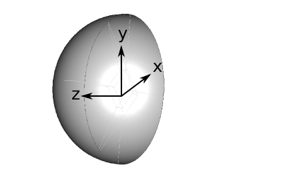
Figure 67 Schematic representation of the sliced sphere
As indicated, a non-uniform temperature profile was used as a thermal boundary condition on the spherical wall. The temperature (\(T\)) was specified as a function of \(x\):
with,
The energy equation in a non-dimensional form [4] for a steady state can be expressed as:
where, \(Gr\) is the Grashof number. Since, \(Ra = Gr~Pr\) the above equation can be rewritten along with expanding the Laplacian term (\(\nabla^2\)) as
where \(\alpha\) is the thermometric conductivity. It is reasonable to assume that (\(1/Ra\)) is approximately equal to the thermometric conductivity (\(\alpha\)), which is given as
where, \(k\), \(\rho\), \(C_p\) and \(\nu\) are the thermal conductivity, density, specific heat capacity and kinematic viscosity of the fluid respectively. Using the above relation with a value of \(Ra = 2000\) and \(Pr = 0.7\), the kinematic viscosity was calculated to be \(\nu = 3.4 \times 10^{-4}~m^2/s\). The coefficient of thermal expansion (\(\beta\)) needed to model the Boussinesq buoyancy term was evaluated from the following relation
where, \(g\) is the acceleration due to gravity and \(D\) is the diameter of the sphere. \(\beta\) was calculated to \(3.567\times10^{-5}~1/K\). In the following table, a summary of the properties are given. Note that gravity acts in \(-y\) direction.
\(Ra\) |
\(Pr\) |
\(T~(K)\) |
\(p~(m^2/s^2)\) |
\(\nu~(m^2/s)\) |
\(\beta~(1/K)\) |
|---|---|---|---|---|---|
\(2000\) |
\(0.7\) |
\(T = x\) |
\((0)\) Gauge |
\(3.4 \times 10^{-4}\) |
\(3.567\times10^{-5}\) |
Although the temperature is calculated in this simulation, a constant viscosity is used. Since the temperature gradient is very small (\(\mathcal{O}(1)\)), effect of temperature on the viscosity would be insignificant. The kinematic definition of pressure is used here.
Computational Domain and Boundary Conditions
The computational domain was a half sphere with an \(x-y\) plane of symmetry at \(z = 0~m\). The surface temperature was prescribed as discussed above. The initialisation of the fluid temperature within the sphere follows that of the surface temperature (\(T = x\)) and is depicted in Figure 68 at the symmetry plane. Note that this figure also aids in providing a clarity of understanding for the temperature variation over the spherical surface.
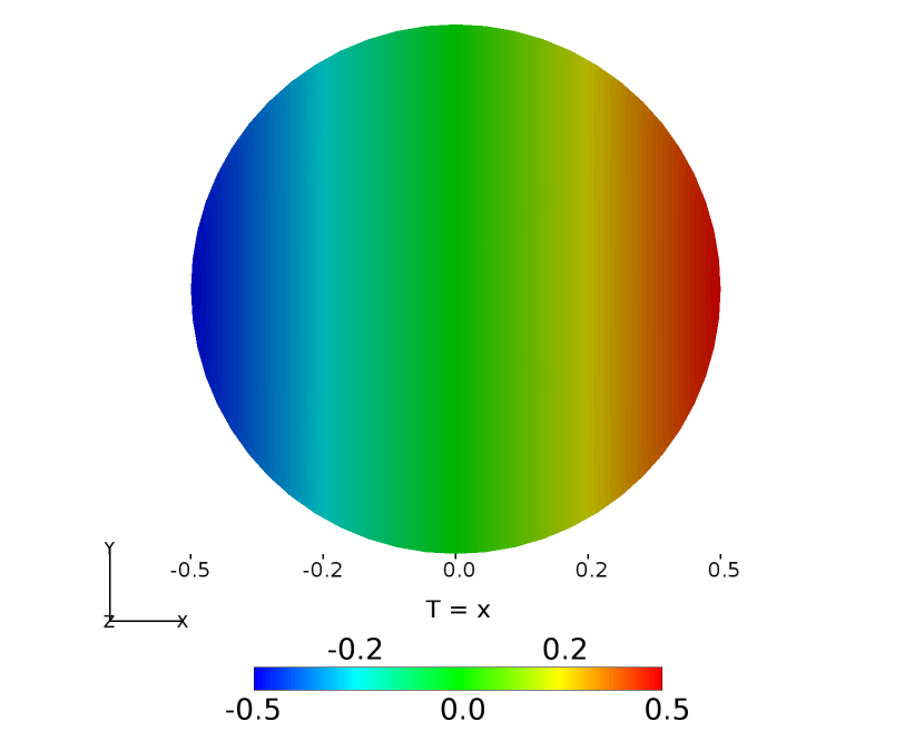
Figure 68 Computational domain and temperature boundary condition
Boundary Conditions and Initialisation
- Wall
Velocity: Fixed uniform velocity \(u, v, w = 0\)
Pressure: Uniform zero Buoyant Pressure
Temperature: Linear unction of \(x\) (\(T = x\))
- Symmetry Plane
Velocity: Symmetry
Pressure: Symmetry
Temperature: Symmetry
- Initialisation
Velocity: Fixed uniform velocity \(u, v, w = 0\)
Pressure: Uniform zero Buoyant Pressure
Temperature: Linear function of \(x\) (\(T = x\))
Computational Grid
The computational grid for the half sphere was generated using Pointwise. A fully structured grid was constructured with a total of 18564 cells. As seen in Figure 69, an O-H topology used where an H-block is centred within 5 O-blocks.
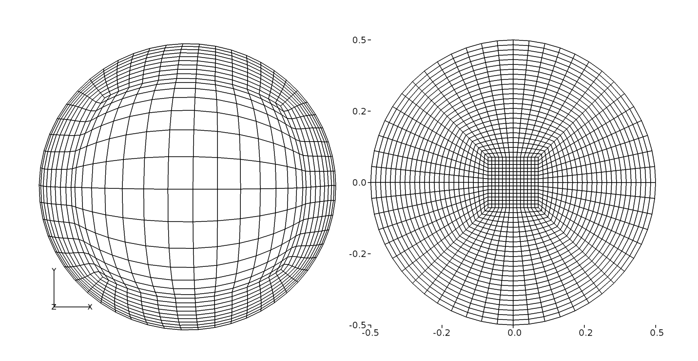
Figure 69 O-grid distribution on the wall and plane of symmetry
Results and Discussion
The steady solution to the natural convection in a buoyant sphere was obtained using Caelus 9.04 with the SLIM solver that includes the a buoyancy source term based on the Boussinesq assumption. Since SLIM is inherently time-accurate, the simulation was run sufficiently long such that a steady state was achieved. In Figure 70, compares the isotherms obtained with SLIM and the analytical isotherms obtained with a first order approximation. Close agreement was observed.
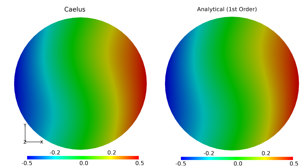
Figure 70 Comparison of temperature isotherms between computational and analytical data
Conclusions
A validation study of a buoyant flow inside a spherically heated cavity was conducted using Caelus 9.04. The isotherms obtained from the CFD results were compared with the first order analytical solution and excellent agreement was observed.