Totorials: Incompressible Turbulent Flow
Turbulent Flat Plate
This tutorial considers the simulation of turbulent incompressible flow over a two-dimensional sharp leading-edge flat plate using Caelus 9.04. Some basic steps to start a Caelus simulation for a turbulent flow environment will be shown such as specifying input data to define the boundary conditions, fluid properties, turbulence parameters and discretization/solver settings. Subsequently, the velocity contour over the plate will be visualised to identify the developed boundary layer. It will be further shown in sufficient detail to carry out Caelus simulation so that the user is able to reproduce accurately.
Objectives
Through this tutorials the user will be familiarised with setting up the Caelus simulation for steady, turbulent, incompressible flow over a sharp leading-edge flat-plate in two-dimensions. Further, the user will also be able to visualise the boundary layer. The following steps are carried out in this tutorial
- Background
A brief description about the problem
Geometry and freestream details
- Grid generation
Computational domain and boundary details
Computational grid generation
Exporting grid to Caelus
- Problem definition
Directory structure
Setting up boundary conditions, physical properties and control/solver attributes
- Execution of the solver
Monitoring the convergence
Writing the log files
- Results
Visualisation of turbulent boundary layer
Pre-requisites
It is assumed that the user is familiar with the Linux command line environment using a terminal or Caelus-console (for Windows OS) and Caelus is installed correctly with appropriate environment variables set. The grid used here is obtained from Turbulence Modeling Resource in a Plot3D format and is exported to Caelus format using Pointwise. However, the user is free to use their choice of grid generation tool to covert the Plot3D file to Caelus format.
Background
Turbulent flow over a flat-plate configuration presents an ideal case to introduce the user with the turbulent simulation using Caelus. Here, the steady-state solution to the incompressible flow over the plate will be obtained, which results in a turbulent boundary layer. The shear stress distribution along the length of the wall and the velocity profile across the wall would be used to infer the development of the turbulent boundary layer. The user can look at the validation section for more details at Zero Pressure Gradient Flat Plate.
The flat-plate length considered for this tutorial is L = 2.0 m and with a unit Reynolds number of \(5 \times 10^6\). Air is used as a fluid and a temperature of T = 300 K is assumed. Based on the Reynolds number and temperature, kinematic viscosity evaluates to \(\nu = 1.38872\times10^{-5}~(m^2/s)\). A freestream velocity of \(U = 69.436113~m/s\) is used. In Figure 26, a schematic of the flat-plate is shown. Note that the 2D plane of interest is in \(x-z\) directions.

Figure 26 Schematic of the flat-plate flow
The freestream conditions that would be used is given in the below table
Fluid |
\(L~(m)\) |
\(Re/L~(1/m)\) |
\(U~(m/s)\) |
\(p~(m^2/s^2)\) |
\(T~(K)\) |
\(\nu~(m^2/s)\) |
|---|---|---|---|---|---|---|
Air |
0.3048 |
\(5 \times 10^6\) |
69.436113 |
Gauge (0) |
300 |
\(1.38872\times10^{-5}\) |
Grid Generation
The hexahedral grid used in this tutorial is obtained from Turbulence Modeling Resource that has 137 X 97 cells in \(x-z\) directions respectively. The original 3D grid is in Plot3D and is then converted to Caelus compatible polyMesh format.
The computational domain is a rectangular block that encompasses the flat-plate. In Figure 27 below, the details of the boundaries in 2D (\(x-z\) plane) that will be used is shown. The region of interest, which is highlighted in blue extends between \(0 \leq x \leq 2.0~m\), where the leading-edge is at \(x=0\). Due to the viscous nature of the flow, the velocity at the wall is zero which is represented through a no-slip boundary wherein \(u,v,w = 0\). Upstream of the leading edge, a symmetry boundary at the wall will be used. The inlet boundary is placed at the start of the symmetry boundary and the outlet is placed at the exit of the flat-plate the no-slip wall. The entire top boundary will be again modelled as a symmetry plane.

Figure 27 Flat-plate computational domain
The polyMesh grid as noted earlier is in 3D. However, since the flow over a flat-plate is two-dimensional, the 2D plane that is considered here is in \(x-z\) directions. It would therefore be ideal to have one-cell thick in the direction (\(y\)), normal to the 2D plane of interest, where the flow is considered symmetry. The two \(x-z\) planes obtained as a result of having 3D grid need boundary conditions to be specified. Since the flow is 2D, we do not need to solve for flow in 3D. This can easily be achieved in Caelus by specifying empty boundary condition for each of the two planes. As a consequence, the flow in \(y\) direction would be symmetry.
Note
A velocity value of \(v=0\) needs to be specified at appropriate boundaries although no flow is solved in the \(y\) direction.
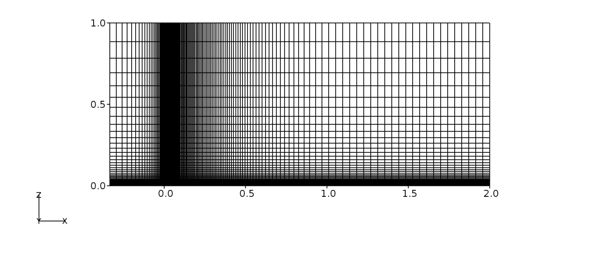
Figure 28 Flat-plate computational grid in \(x-z\) plane
In Figure 28, the 2D grid is shown which has 137 X 97 cells in \(x-z\) directions respectively. To capture the turbulent boundary layer accurately, the grids are refined close to the wall and \(y^+\) is estimated to be less than 1. Due to this, no wall-functions would be used to estimate the velocity gradients near the wall and integration is carried up to the wall.
Problem definition
In this section, several key instructions would be provided to set-up the turbulent flat-plate problem along with details of file configuration. A full working case can be found in:
/tutorials/incompressible/simpleSolver/ras/ACCM_flatPlate2D
However,the user is free to start the case setup from scratch consistent with the directory stucture discussed below.
Directory Structure
Note
All commands shown here are entered in a terminal window, unless otherwise mentioned
For setting up the problem, we need to further have few more sub-directories where relevant files can be created. Caelus requires time, constant and system sub-directories. Since we will begin the simulation at time \(t = 0~s\), the time sub-directory should be just 0.
In the 0 sub-directory, additional files are required for specifying the boundary properties. The following table lists the necessary files required based on the turbulence model chosen.
Parameter |
File name |
|---|---|
Pressure (\(p\)) |
|
Velocity (\(U\)) |
|
Turbulent viscosity (\(\nu\)) |
|
Turbulence field variable (\(\tilde{\nu}\)) |
|
Turbulent kinetic energy (\(k\)) |
|
Turbulent dissipation rate (\(\omega\)) |
|
As can be noted from the above table, we will be considering two turbulence models namely, Spalart-Allmaras (SA) and \(k-\omega\) - Shear Stress Transport (\(\rm{SST}\)) in the current exercise. These files set the dimensions, initialisation and boundary conditions to the problem, which also forms the three principle entries required.
The user should take into account that Caelus is case sensitive and therefore where applicable, the directory set-up should be identical to what is shown here.
Boundary Conditions and Solver Attributes
Boundary Conditions
Initially, let us set-up the boundary conditions. Referring back to Fig. %s:num:t-fp-domain-tutorials, the following are the boundary conditions that will be specified:
- Inlet
Velocity: Fixed uniform velocity \(u = 69.436113~m/s\) in \(x\) direction
Pressure: Zero gradient
Turbulence:
Spalart–Allmaras (Fixed uniform values of \(\nu_{t~\infty}\) and \(\tilde{\nu}_{\infty}\) as given in Turbulence freestream conditions for SA model)
\(k-\omega~\textrm{SST}\) (Fixed uniform values of \(k_{\infty}\), \(\omega_{\infty}\) and \(\nu_{t~\infty}\) as given in Turbulence freestream conditions for k-\omega~\rm{SST} model)
- Symmetry
Velocity: Symmetry
Pressure: Symmetry
Turbulence: Symmetry
- No-slip wall
Velocity: Fixed uniform velocity \(u, v, w = 0\)
Pressure: Zero gradient
Turbulence:
Spalart–Allmaras (Fixed uniform values of \(\nu_{t}=0\) and \(\tilde{\nu}=0\))
\(k-\omega~\textrm{SST}\) (Zero gradient \(k\) and \(\omega\); Calculated \(\nu_t=0\); )
- Outlet
Velocity: Zero gradient velocity
Pressure: Fixed uniform gauge pressure \(p = 0\)
Turbulence:
Spalart–Allmaras (Calculated \(\nu_{t}=0\) and Zero gradient \(\tilde{\nu}\))
\(k-\omega~\textrm{SST}\) (Zero gradient \(k\) and \(\omega\); Calculated \(\nu_t=0\); )
- Initialisation
Velocity: Fixed uniform velocity \(u = 69.436113\) in \(x\) direction
Pressure: Zero Gauge pressure
Turbulence:
Spalart–Allmaras (Fixed uniform values of \(\nu_{t~\infty}\) and \(\tilde{\nu}_{\infty}\) as given in Turbulence freestream conditions for SA model)
\(k-\omega~\textrm{SST}\) (Fixed uniform values of \(k_{\infty}\), \(\omega_{\infty}\) and \(\nu_{t~\infty}\) as given in Turbulence freestream conditions for k-\omega~\rm{SST} model)
Starting with the pressure, let us open p using a text editor, which has the following contents.
/*---------------------------------------------------------------------------*\
Caelus 9.04
 Web:      www.caelus-cml.com
\*---------------------------------------------------------------------------*/
FoamFile
{
    version     2.0;
    format      ascii;
    class       volScalarField;
    location    "0";
    object      p;
}
// * * * * * * * * * * * * * * * * * * * * * * * * * * * * * * * * * * * * * //

dimensions      [0 2 -2 0 0 0 0];

internalField   uniform 0;

boundaryField
{
    bottom
    {
        type            symmetryPlane;
    }
    inflow
    {
        type            zeroGradient;
    }
    left
    {
        type            empty;
    }
    outflow
    {
        type            fixedValue;
        value           uniform 0;
    }
    right
    {
        type            empty;
    }
    top
    {
        type            symmetryPlane;
    }
    wall
    {
        type            zeroGradient;
    }
}


// ************************************************************************* //
As can be seen, the above file begins with a dictionary named FoamFile which contains the standard set of keywords for version, format, location, class and object names.
dimensionis used to specify the physical dimensions of the pressure field. Here, pressure is defined in terms of kinematic pressure with the units (\(m^2/s^2\)) written as
[0 2 -2 0 0 0 0]
internalFieldis used to specify the initial conditions. It can be either uniform or non-uniform. Since we have a 0 initial uniform gauge pressure, the entry is
uniform 0;
boundaryFieldis used to specify the boundary conditions. In this case its the boundary conditions for pressure at all the boundary patches.
In a similar approach, let us open the file U.
/*---------------------------------------------------------------------------*\
Caelus 9.04
 Web:      www.caelus-cml.com
\*---------------------------------------------------------------------------*/
FoamFile
{
    version     2.0;
    format      ascii;
    class       volVectorField;
    location    "0";
    object      U;
}
// * * * * * * * * * * * * * * * * * * * * * * * * * * * * * * * * * * * * * //

dimensions      [0 1 -1 0 0 0 0];

internalField   uniform (69.4361 0 0);

boundaryField
{
    bottom
    {
        type            symmetryPlane;
    }
    inflow
    {
        type            fixedValue;
        value           uniform (69.4361 0 0);
    }
    left
    {
        type            empty;
    }
    outflow
    {
        type            zeroGradient;
    }
    right
    {
        type            empty;
    }
    top
    {
        type            symmetryPlane;
    }
    wall
    {
        type            noSlipWall;
    }
}


// ************************************************************************* //
As detailed above, the principle entries for velocity field are self explanatory and the dimensions are typically for that of velocity with the units \(m/s\) ([0 1 -1 0 0 0 0]). Since we initialise the flow with a uniform freestream velocity, we set the internalField to uniform (69.4361 0 0) which represents three components of velocity. Similarly, inflow boundary patch has three velocity components.
Similarly, the turbulent properties needed at the boundaries can be set. We begin with opening the file nut, which is the turbulent kinematic viscosity and is shown below.
/*---------------------------------------------------------------------------*\
Caelus 9.04
 Web:      www.caelus-cml.com
\*---------------------------------------------------------------------------*/
FoamFile
{
    version     2.0;
    format      ascii;
    class       volScalarField;
    location    "0";
    object      nut;
}
// * * * * * * * * * * * * * * * * * * * * * * * * * * * * * * * * * * * * * //

dimensions      [0 2 -1 0 0 0 0];

internalField   uniform 2.9224e-06;

boundaryField
{
    bottom
    {
        type            symmetryPlane;
    }
    inflow
    {
        type            fixedValue;
        value           uniform 2.9224023e-06;
    }
    left
    {
        type            empty;
    }
    outflow
    {
        type            calculated;
        value           uniform 0;
    }
    right
    {
        type            empty;
    }
    top
    {
        type            symmetryPlane;
    }
    wall
    {
        type            fixedValue;
        value           uniform 0;
    }
}


// ************************************************************************* //
Here, the turbulent viscosity is specified as kinematic and therefore the units are \(m^2/s\) ([0 2 -1 0 0 0 0] ). The value of turbulence viscosity at freestream, specified at inflow patch is calculated as detailed in Turbulence freestream conditions for SA model and Turbulence freestream conditions for k-\omega~\rm{SST} model for SST models respectively and is specified accordingly. The same value also goes for internalField. Note that a fixedValue of 0 is used for the wall which suggests that on the wall, it is only the molecular (laminar) viscosity that prevails.
We shall now look at nuTilda which is a turbulence field variable, specific to the SA model and has same units ([0 2 -1 0 0 0 0]) as kinematic turbulent viscosity. The details of which are given in Turbulence freestream conditions for SA model. In the file nuTilda, the entries specified for the boundaryField are identical to that of turbulent kinematic viscosity explained above.
/*---------------------------------------------------------------------------*\
Caelus 9.04
 Web:      www.caelus-cml.com
\*---------------------------------------------------------------------------*/
FoamFile
{
    version     2.0;
    format      ascii;
    class       volScalarField;
    location    "0";
    object      nuTilda;
}
// * * * * * * * * * * * * * * * * * * * * * * * * * * * * * * * * * * * * * //

dimensions      [0 2 -1 0 0 0 0];

internalField   uniform 4.166166e-05;

boundaryField
{
    bottom
    {
        type            symmetryPlane;
    }
    inflow
    {
        type            fixedValue;
        value           uniform 4.166166e-05;
    }
    left
    {
        type            empty;
    }
    outflow
    {
        type            zeroGradient;
    }
    right
    {
        type            empty;
    }
    top
    {
        type            symmetryPlane;
    }
    wall
    {
        type            fixedValue;
        value           uniform 0;
    }
}


// ************************************************************************* //
We now proceed to files k and omega, specific to only \(k-\omega~\rm{SST}\) model. As we know, \(k-\omega~\rm{SST}\) is a turbulence model which solves for the turbulent kinetic energy and the specific rate of dissipation using two partial differential equations. Caelus therefore requires information about these to be specified when this model is used. Firstly, the file k with the following contents is needed.
/*---------------------------------------------------------------------------*\
Caelus 9.04
 Web:      www.caelus-cml.com
\*---------------------------------------------------------------------------*/
FoamFile
{
    version     2.0;
    format      ascii;
    class       volScalarField;
    location    "0";
    object      k;
}
// * * * * * * * * * * * * * * * * * * * * * * * * * * * * * * * * * * * * * //

dimensions      [0 2 -2 0 0 0 0];

internalField   uniform 0.0010848;

boundaryField
{
    bottom
    {
        type            symmetryPlane;
    }
    inflow
    {
        type            fixedValue;
        value           uniform 0.0010848;
    }
    left
    {
        type            empty;
    }
    outflow
    {
        type            zeroGradient;
    }
    right
    {
        type            empty;
    }
    top
    {
        type            symmetryPlane;
    }
    wall
    {
        type            fixedValue;
        value           uniform 1e-10;
    }
}


// ************************************************************************* //
The unit of kinetic energy is \(m^2/s^2\) and this is set in dimensions as [0 2 -2 0 0 0 0]. As with other turbulent quantities discussed above, the value of \(k\) (refer Turbulence freestream conditions for k-\omega~\rm{SST} model needs to be specified for internalField, inflow and wall. Please note that for wall boundaryField with no wall-function, a small, non-zero fixedValue is required.
Next, the value for \(\omega\) is evaluated in omega file as shown below and as detailed in Turbulence freestream conditions for k-\omega~\rm{SST} model.
/*---------------------------------------------------------------------------*\
Caelus 9.04
 Web:      www.caelus-cml.com
\*---------------------------------------------------------------------------*/
FoamFile
{
    version     2.0;
    format      ascii;
    class       volScalarField;
    location    "0";
    object      omega;
}
// * * * * * * * * * * * * * * * * * * * * * * * * * * * * * * * * * * * * * //

dimensions      [0 0 -1 0 0 0 0];

internalField   uniform 8679.5135;

boundaryField
{
    bottom
    {
        type            symmetryPlane;
    }
    inflow
    {
        type            fixedValue;
        value           uniform 8679.5135;
    }
    left
    {
        type            empty;
    }
    outflow
    {
        type            zeroGradient;
    }
    right
    {
        type            empty;
    }
    top
    {
        type            symmetryPlane;
    }
    wall
    {
        type            omegaWallFunction;
        value           uniform 1;
    }
}


// ************************************************************************* //
The unit of specific rate of dissipation for \(\omega\) is \(1/s\) which is set in dimensions as [0 0 -1 0 0 0 0]. The internalField and inflow gets a fixedValue. Note that for wall boundaryField, we specify omegaWallFunction and this is a model requirement and sets omega to the correct value near wall based on the \(y^+\). In conjunction, the value that goes with omegaWallFunction can be anything and for simplicity its set to 1.
Before setting up other parameters, it is important to ensure that the boundary conditions (inflow, outflow, top, etc) specified in the above files should be the grid boundary patches (surfaces) generated by the grid generation tools and their names are identical. Further, the two boundaries in \(x-z\) plane named here as left and right have empty boundary conditions which forces Caelus to assume the flow to be in 2D. With this, the setting up of boundary conditions are completed.
Grid file and Physical Properties
The turbulent flat-plate grid files is placed in the constant/polyMesh sub-directory. Additionally, the physical properties are specified in various different files present in the directory constant.
As you can see in the constant directory, three files are listed in addition to the polyMesh sub-directory. In the first file, RASProperties, the Reynolds-Average-Stress (RAS) model is specified as below. Note that depending on the turbulence model you wish to run with, the line that corresponds to that specific model should be enabled
/*-------------------------------------------------------------------------------*
Caelus 9.04
Web:   www.caelus-cml.com
\*------------------------------------------------------------------------------*/

FoamFile
{
	version				2.0;
	format				ascii;
	class				dictionary;
	location			"constant";
	object				RASProperties;
}

//--------------------------------------------------------------------------------

// For Spalarat-Alamaras Model, enable the below line
RASModel				SpalartAllmaras;

// For k-omega SST Model, enable the below line
// RASModel				kOmegaSST;

turbulence				on;

printCoeffs				on;
Next, we look at the transportProperties file, where transport model and kinematic viscosity is specified.
/*-------------------------------------------------------------------------------*
Caelus 9.04
Web:   www.caelus-cml.com
\*------------------------------------------------------------------------------*/

FoamFile
{
	version				2.0;
	format				ascii;
	class				dictionary;
	location			"constant";
	object				transportProperties;
}

//--------------------------------------------------------------------------------

transportModel				Newtonian;

nu					nu [0 2 -1 0 0 0 0] 1.388722E-5;
As the viscous behaviour is Newtonian, the transportModel is given using the keyword Newtonian and the value of molecular (laminar) kinematic viscosity (nu) is given having the units \(m^2/s\) ([0 2 -1 0 0 0 0]).
The final file in this class is the turbulenceProperties file, which sets the simulationType to RASModel. Both SA and \(k-\omega~\rm{SST}\) are classified as Reynolds Average Stress (RAS) models.
/*-------------------------------------------------------------------------------*
Caelus 9.04
Web:   www.caelus-cml.com
\*------------------------------------------------------------------------------*/

FoamFile
{
	version				2.0;
	format				ascii;
	class				dictionary;
	location			"constant";
	object				turbulenceProperties;
}

//--------------------------------------------------------------------------------

simulationType				RASModel;
Controls and Solver Attributes
In this section, the files required to control the simulation and specifying the type of discretization method along with the linear solver settings are provided. These are placed in the system directory.
First, we begin with the controlDict file as below
/*-------------------------------------------------------------------------------*
Caelus 9.04
Web:   www.caelus-cml.com
\*------------------------------------------------------------------------------*/

FoamFile
{
	version				2.0;
	format				ascii;
	class				dictionary;
	location			"system";
	object				controlDict;
}

//-------------------------------------------------------------------------------

application				simpleSolver;

startFrom				startTime;

startTime				0;

stopAt					endTime;

endTime					20000;

deltaT					1;

writeControl				runTime;

writeInterval				1000;

purgeWrite				0;

writeFormat				ascii;

writePrecision				12;

writeCompression			true;

timeFormat				general;

timePrecision				6;

runTimeModifiable			true;

//-------------------------------------------------------------------------------

// Function Objects to obtain forces

functions
{
	forces
	{
		type			forces;

        functionObjectLibs	("libforces.so");
        patches     		( wall );
        CofR      			(0 0 0);
        rhoName         	rhoInf;
        rhoInf          	1.347049;
        writeControl   	    timeStep;
        writeInterval  	    50;
     }
}
As can be noted in the above file, simpleSolver solver is used and the simulation begins at t = 0 s. This logically explains the need for 0 directory where the data files are read at the beginning of the run. Therefore, the keyword startFrom is set to startTime, where startTime would be 0. Since the simulation is steady-state we specify the total number of iterations as a keyword for endTime. Via the writeControl and writeInternal keywords, the interval at which the solutions are saved can be specified. Also included is the function object to obtain the force over the wall every 50 iterations. Note that for obtaining the force, the freestream density (rhoInf) is required and is specified with the value.
The discretization schemes for the finite volume discretization that will be used is set through the fvSchemes file shown below
/*-------------------------------------------------------------------------------*
Caelus 9.04
Web:   www.caelus-cml.com
\*------------------------------------------------------------------------------*/

FoamFile
{
	version				2.0;
	format				ascii;
	class				dictionary;
	object				fvSchemes;
}

//------------------------------------------------------------------------------

ddtSchemes
{
	default				steadyState;
}

gradSchemes
{
	default				Gauss	linear;
	grad(p)				Gauss	linear;
	grad(U)				Gauss	linear;
}

divSchemes
{
	default				none;
	div(phi,U)			Gauss	linearUpwind	grad(U);
	div(phi,nuTilda)		Gauss	upwind;	// Will be used for S-A model only
	div(phi,k)			Gauss 	upwind; // will be used for k-epsilon & k-omega only
	div(phi,omega)			Gauss 	upwind;	// Will be used for k-omega model only
	div((nuEff*dev(T(grad(U)))))	Gauss   linear;
	div(phi,symm(grad(U))) 		Gauss 	linear;

}

laplacianSchemes
{
	default				none;
	laplacian(nu,U)			Gauss 	linear 	corrected;
	laplacian(nuEff,U)		Gauss 	linear 	corrected;
	laplacian(DnuTildaEff,nuTilda) 	Gauss 	linear 	corrected; // Will be used for S-A model only
	laplacian(DkEff,k)		Gauss 	linear 	corrected; // Will be used for k-omega & k-omega only
	laplacian(DomegaEff,omega)	Gauss 	linear 	corrected; // Will be used for k-omega model only
	laplacian(rAUf,p)		Gauss 	linear	corrected;
	laplacian(1,p)			Gauss 	linear 	corrected;
}

interpolationSchemes
{
	default				linear;
	interpolate(HbyA)		linear;
}

snGradschemes
{
	default				corrected;
}
The linear solver controls and tolerances are set in fvSolution as given below
/*-------------------------------------------------------------------------------*
Caelus 9.04
Web:   www.caelus-cml.com
\*------------------------------------------------------------------------------*/
FoamFile
{
        version                         2.0;
        format                          ascii;
        class                           dictionary;
        location                        "system";
        object                          fvSolution;
}

//------------------------------------------------------------------------------

solvers
{
        p
        {
                solver                  PCG;
                preconditioner          SSGS;
                tolerance               1e-8;
                relTol                  0.01;
        }
        U
        {
                solver                  PBiCGStab;
                preconditioner          USGS;
                tolerance               1e-7;
                relTol                  0.01;
        }

        "(k|omega|nuTilda)"
        {
                solver                  PBiCGStab;
                preconditioner          USGS;
                tolerance               1e-08;
                relTol                  0;
        }
}

SIMPLE
{
        nNonOrthogonalCorrectors        1;
        pRefCell                        0;
        pRefValue                       0;
}

// relexation factors

relaxationFactors
{
        p                               0.3;
        U                               0.5;
        nuTilda                         0.5;
        k                               0.5;
        omega                           0.5;
}
Here, different linear solvers are used to solve velocity, pressure and turbulence quantities. We also set the nNonOrthogonalCorrectors to 1 in this case. Further, relaxation is set on the primary and turbulent variables so that the solution is more stable. Furthermore, the relTol is not set to 0 unlike a time-accurate set-up. This is because we are solving for a steady-state solution and a very low (\(\approx 0\)) tolerance at every iteration is not required as the entire system of equations converges to the global tolerance set as the simulation progresses to steady state.
Now the set-up of the directory structure with all the relevant files the directory tree should appear identical to the one shown below
.
├── 0
│   ├── epsilon
│   ├── k
│   ├── nut
│   ├── nuTilda
│   ├── omega
│   ├── p
│   └── U
├── constant
│   ├── polyMesh
│   │   ├── boundary
│   │   ├── faces
│   │   ├── neighbour
│   │   ├── owner
│   │   └── points
│   ├── RASProperties
│   ├── transportProperties
│   └── turbulenceProperties
└── system
    ├── controlDict
    ├── fvSchemes
    └── fvSolution
Execution of the solver
Prior to execution of solver, renumbering of the grid/mesh needs to be performed in addition to checking the quality of the grid/mesh. Renumbering the grid-cell list is vital to reduce the matrix bandwidth while quality check gives us the mesh statistics. Renumbering and mesh quality can be determined by executing the following from the top directory.
caelus run -- renumberMesh -overwrite
caelus run -- checkMesh
At this stage, it is suggested that the user should take note of the matrix bandwidth before and after the mesh renumbering. When the checkMesh is performed, the mesh statistics are shown as below
/*---------------------------------------------------------------------------*\
 Caelus 8.04
 Web:      www.caelus-cml.com
\*---------------------------------------------------------------------------*/
// * * * * * * * * * * * * * * * * * * * * * * * * * * * * * * * * * * * * * //

Checking geometry...
    Overall domain bounding box (-0.06 0 0.03) (1.2192 0.15 0.055)
    Mesh (non-empty, non-wedge) directions (1 1 0)
    Mesh (non-empty) directions (1 1 0)
    All edges aligned with or perpendicular to non-empty directions.
    Boundary openness (5.80542e-19 1.1194e-17 1.1403e-14) OK.
    Max cell openness = 2.2093e-16 OK.
    Max aspect ratio = 55.555 OK.
    Minimum face area = 1e-08. Maximum face area = 0.000138887.  Face area magnitudes OK.
    Min volume = 2.5e-10. Max volume = 2.50831e-07.  Total volume = 0.004797.  Cell volumes OK.
    Mesh non-orthogonality Max: 0 average: 0
    Non-orthogonality check OK.
    Face pyramids OK.
    Mesh skewness Max: 3.85044e-13 average: 9.40402e-15 OK.
    Coupled point location match (average 0) OK.

Mesh OK.

End
In the above terminal output, we get Failed 1 mesh checks. and this is because of the high aspect ratio meshes present immediate to the wall due to very low (\(<< 1~y^+\)). However, Caelus can solve on this mesh. The next step is to execute the solver and monitoring the progress of the solution. The solver is always executed from the top directory.
caelus run -l my-turbulent-flat-plate.log -- simpleSolver
With the execution of the above command, the simulation begins and the progress of the solution is written to the specified log file (my-turbulent-flat-plate.log). The log file can be further processed to look at the convergence history and this can be done as follows
caelus logs -w my-turbulent-flat-plate.log
This allows you to look at the convergence of different variables with respect to the number of iterations carried out. In Fig. %s:num:tfpconvergencetutorials pressure convergence is shown.
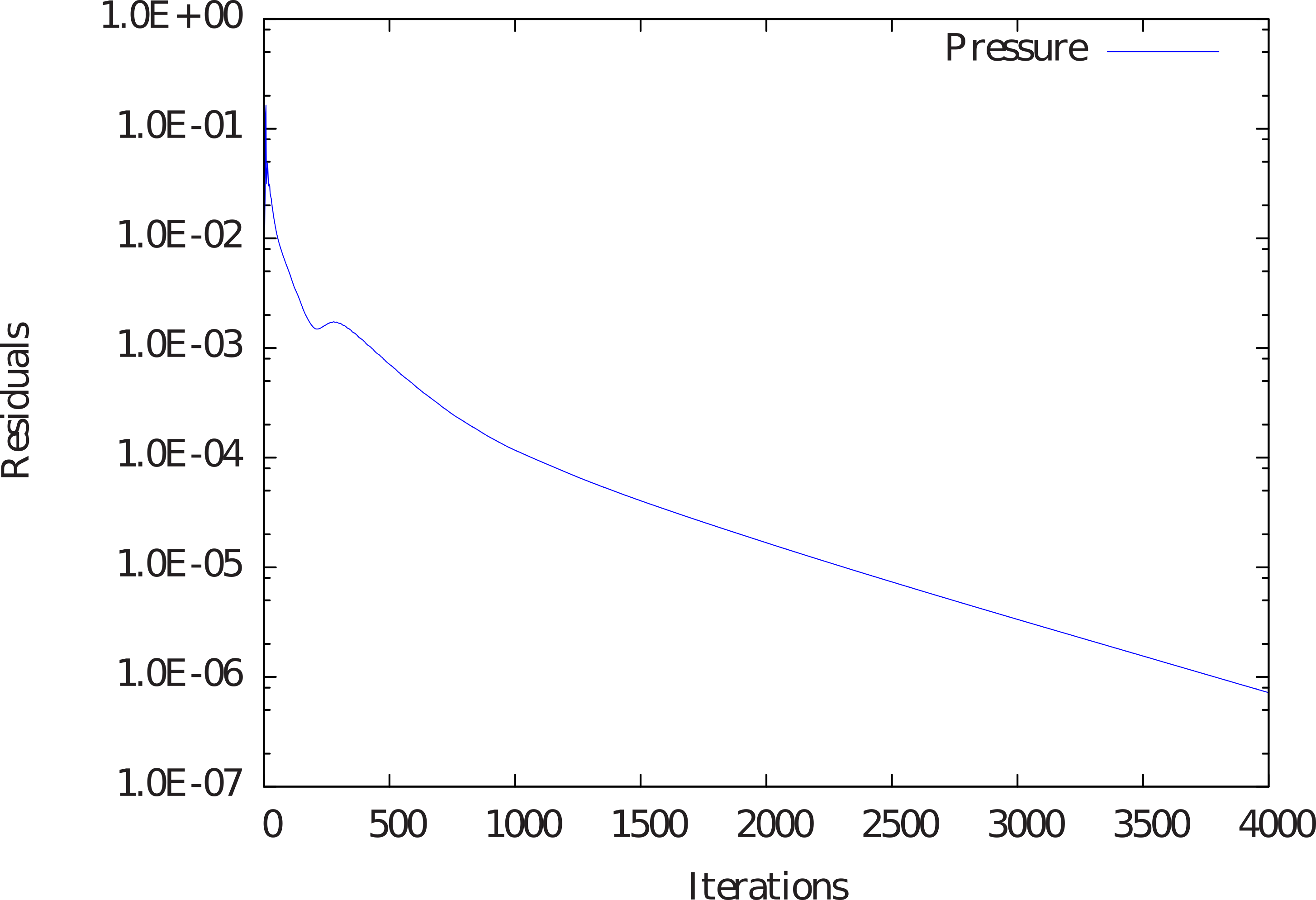
Figure 29 Convergence of pressure with respect to iterations
Results
The turbulent flow over the flat plate is shown here through velocity magnitude contours for SA model. In Fig. %s:num:tfpvelocitytutorials the boundary layer over the entire flat-plate and in the region up to \(x=0.10~m\) is emphasised. The growth of the boundary layer can be seen very clearly. Since the Reynolds number of the flow is reasonably high, the turbulent boundary layer seems thin in comparison to the length of the plate.
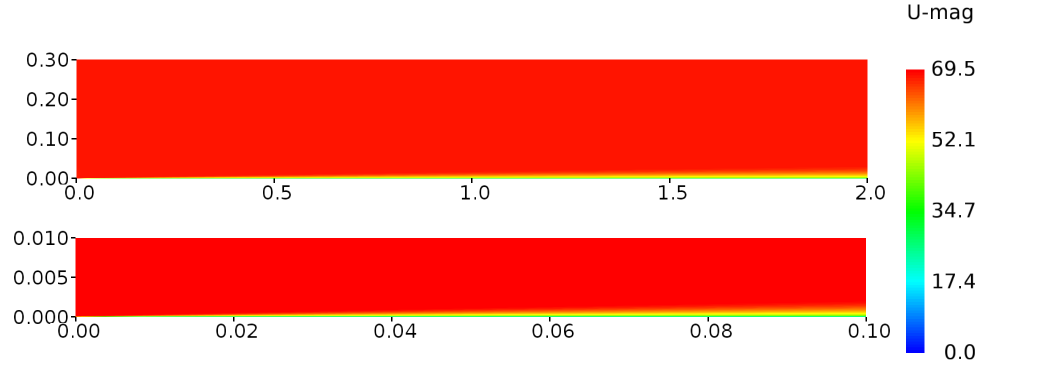
Figure 30 Contour of velocity magnitude over the flat-plate
Bump in a Channel
The simulation of turbulent flow over a two-dimensional bump in a channel is considered in this tutorial and will be performed using Caelus 9.04. As with the other tutorials, setting up the directory structure, fluid properties, boundary conditions, turbulence properties etc will be shown. Further to this, visualisation of the solution will be shown to look at the velocity and pressure contours over the bump surface. These steps would be shown in sufficient details so that the user is able to reproduce the tutorial accurately.
Objectives
Some of the main objectives of this tutorial would be for the user to get familiarise with setting up the Caelus simulation for steady, turbulent, incompressible flow over a two-dimensional bump in a channel and be able to post-process the desired solution. Following would be some of the steps that would be covered.
- Background
A brief description about the problem
Geometry and freestream details
- Grid generation
Computational domain and boundary details
Computational grid generation
Exporting grid to Caelus
- Problem definition
Directory structure
Setting up boundary conditions, physical properties and control/solver attributes
- Execution of the solver
Monitoring the convergence
Writing the log files
- Results
Visualisation of flow near the bump
Pre-requisites
The user should be familiar with a Linux command line environment via a terminalor caelus-console (For Windows OS). It is also assumed that Caelus is installed correctly with appropriate environment variables set. The grid used here is obtained from Turbulence Modeling Resource in a Plot3D format and is exported to Caelus format using Pointwise. However, the user is free to use their choice of grid generation tool to covert the Plot3D file to Caelus format.
Background
Turbulent flow over a bump in a channel is quite similar to a flat-plate flow, except that due to the curvature effect, a pressure gradient is developed. The flow would be assumed to be steady-state and incompressible. To demonstrate the effect of curvature, the skin friction distribution along the bump will be plotted. For further information on this case, the user can refer to Two-dimensional Bump in a Channel.
The bump, as shown in the schematic below in Figure 31 has a upstream and a downstream flat-plate region that begins at x = 0 m and x = 1.5 m respectively, which gives a total length of L = 1.5 m. The flow has a unit Reynolds number of \(3 \times 10^6\) and Air is used as a fluid with a temperature of 300 K. Based on these values, kinematic viscosity can be evaluated to \(\nu = 2.314537 \times 10^{-5} m^2/s\). To match the required Reynolds number, a freestream velocity of U = 69.436 m/s would be used. Note that the two-dimensional plane considered here is in \(x-z\) directions.
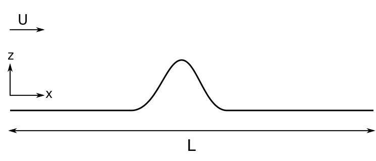
Figure 31 Schematic of the 2D bump
The freestream conditions that will be used is given in the below table (Freestream conditions)
Fluid |
\(L~(m)\) |
\(Re/L~(1/m)\) |
\(U~(m/s)\) |
\(p~(m^2/s^2)\) |
\(T~(K)\) |
\(\nu~(m^2/s)\) |
|---|---|---|---|---|---|---|
Air |
1.5 |
\(3 \times 10^6\) |
69.436113 |
Gauge (0) |
300 |
\(2.314537\times10^{-5}\) |
Grid Generation
The hexahedral grid used in this tutorial is obtained from Turbulence Modeling Resource that contains 704 X 320 cells in \(x-z\) directions respectively. The grid originally is in Plot3D format and is converted to Caelus compatible polyMesh format.
The computational domain is a rectangular channel encompassing the bump. Figure 32 shown below identifies the boundary conditions in a two-dimensional plane (\(x-z\)). The bump region, highlighted in blue extends between \(0 \leq x \leq 1.5~m\), where the velocity at the wall is zero, wherein \(u,v,w=0\) represented through a no-slip boundary. Upstream and downstream of the bump, a symmetry boundary at the wall is used. The inlet and outlet are placed at the end of the symmetry as depicted in the figure and the top boundary has a symmetry condition.
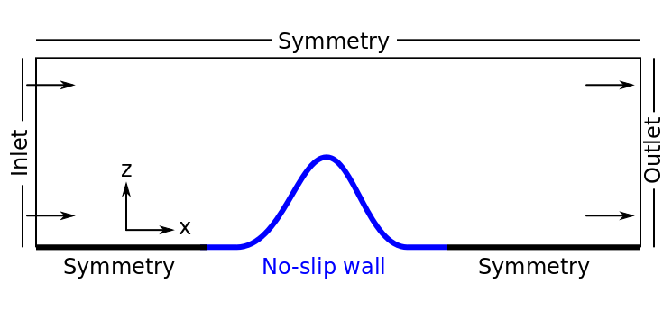
Figure 32 Computational domain of a 2D bump
The polyMesh grid obtained from the conversion of Plot3D is in 3D. However, the flow over a bump is two-dimensional and is solved in a 2D plane with \(x-z\) directions. Therefore, ideally we can have cells with one-cell thick in the direction (\(y\)), normal to the 2D plane, where the flow can be assumed to be symmetry. The two \(x-z\) planes obtained as a result of having a 3D grid require boundary conditions to be specified. As the flow is assumed to be 2D, we do not need to solve the flow in 3D and this can easily be achieved in Caelus by specifying empty boundary condition for each of the two planes. This consequently allows for the flow in \(y\) direction to be symmetry.
Note
A velocity value of \(v=0\) needs to be specified at appropriate boundaries although no flow is solved in the \(y\) direction.
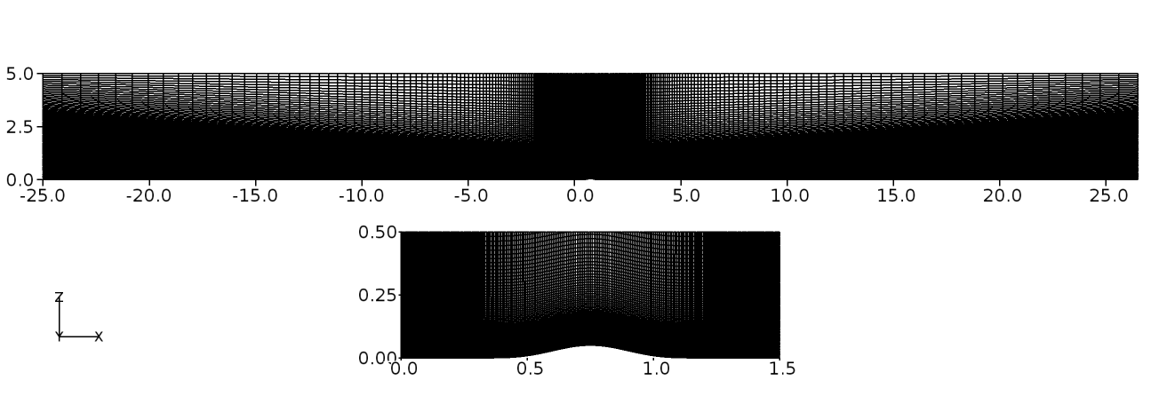
Figure 33 Computational grid of a two-dimensional bump in \(x-z\) plane
In Figure 33 above, the 2D grid is shown with a distribution of 704 X 320 in \(x-z\) directions respectively. The inset focuses the distribution in the region between \(0 \leq x \leq 1.5~m\). As can be seen, the distribution of the grids in the flow normal direction is finer near the wall to capture the turbulent boundary layer more accurately and it is estimated that \(y^+\) is less than 1 for the chosen grid and therefore, no wall-function has been used and the integration is carried out up to the wall.
Problem definition
This section deals with several key instructions need to set-up the turbulent flow over a bump. A full working case of this can be found in:
/tutorials/incompressible/simpleSolver/ras/ACCM_bump2D/
The user is free to start the case setup from scratch consistent with the directory stucture discussed below.
Directory Structure
Note
All commands shown here are entered in a terminal window, unless otherwise mentioned
In order to set-up the problem Caelus requires time, constant and system sub-directories within the main working directory. Typically, the simulations are started at time \(t = 0~s\), which requires a time sub-directory to be 0.
Within the 0 sub-directory, additional files specifying the boundary properties are present. The below table lists the necessary files required based
on the turbulence model chosen
Parameter |
File name |
|---|---|
Pressure (\(p\)) |
|
Velocity (\(U\)) |
|
Turbulent viscosity (\(\nu\)) |
|
Turbulence field variable (\(\tilde{\nu}\)) |
|
Turbulent kinetic energy (\(k\)) |
|
Turbulent dissipation rate (\(\omega\)) |
|
In this tutorial, we will be considering two turbulence models namely, Spalart-Allmaras (SA) and \(k-\omega\) - Shear Stress Transport (\(\rm{SST}\)). The contents of the files listed above sets the dimensions, initialisation and boundary conditions to the defining problem, which also
forms three principle entries required. Firstly, we begin with looking at these files in the 0 sub-directory
The user should take into account that Caelus is case sensitive and therefore the directory set-up should be identical to what is shown here.
Boundary Conditions and Solver Attributes
Boundary Conditions
Referring back to Figure 32, the following are the boundary conditions that will be specified:
- Inlet
Velocity: Fixed uniform velocity \(u = 69.436113~m/s\) in \(x\) direction
Pressure: Zero gradient
Turbulence:
Spalart–Allmaras (Fixed uniform values of \(\nu_{t~\infty}\) and \(\tilde{\nu}_{\infty}\) as given in Turbulence freestream conditions for SA model)
\(k-\omega~\rm{SST}\) (Fixed uniform values of \(k_{\infty}\), \(\omega_{\infty}\) and \(\nu_{t~\infty}\) as given in Turbulence freestream conditions for k-\omega~\rm{SST} model)
- Symmetry
Velocity: Symmetry
Pressure: Symmetry
Turbulence: Symmetry
- No-slip wall
Velocity: Fixed uniform velocity \(u, v, w = 0\)
Pressure: Zero gradient
Turbulence:
Spalart–Allmaras (Fixed uniform values of \(\nu_{t}=0\) and \(\tilde{\nu}=0\))
\(k-\omega~\rm{SST}\) (Fixed uniform values of \(k =<<0\) and \(\nu_t=0\); \(\omega\) = omegaWallFunction)
- Outlet
Velocity: Zero gradient velocity
Pressure: Fixed uniform gauge pressure \(p = 0\)
Turbulence:
Spalart–Allmaras (Calculated \(\nu_{t}=0\) and Zero gradient \(\tilde{\nu}\))
\(k-\omega~\rm{SST}\) (Zero gradient \(k\) and \(\omega\); Calculated \(\nu_t=0\); )
- Initialisation
Velocity: Fixed uniform velocity \(u = 69.436113\) in \(x\) direction
Pressure: Zero Gauge pressure
Turbulence:
Spalart–Allmaras (Fixed uniform values of \(\nu_{t~\infty}\) and \(\tilde{\nu}_{\infty}\) as given in Turbulence freestream conditions for SA model)
\(k-\omega~\rm{SST}\) (Fixed uniform values of \(k_{\infty}\), \(\omega_{\infty}\) and \(\nu_{t~\infty}\) as given in Turbulence freestream conditions for k-\omega~\rm{SST} model)
We begin with p, the pressure file using a text editor with the following content
/*---------------------------------------------------------------------------*\
Caelus 9.04
 Web:      www.caelus-cml.com
\*---------------------------------------------------------------------------*/
FoamFile
{
    version     2.0;
    format      ascii;
    class       volScalarField;
    location    "0";
    object      p;
}
// * * * * * * * * * * * * * * * * * * * * * * * * * * * * * * * * * * * * * //

dimensions      [0 2 -2 0 0 0 0];

internalField   uniform 0;

boundaryField
{
    bottom
    {
        type            symmetryPlane;
    }
    inflow
    {
        type            zeroGradient;
    }
    left
    {
        type            empty;
    }
    outflow
    {
        type            fixedValue;
        value           uniform 0;
    }
    right
    {
        type            empty;
    }
    top
    {
        type            symmetryPlane;
    }
    wall
    {
        type            zeroGradient;
    }
}


// ************************************************************************* //
From the above information, it can be seen that the file begins with a dictionary named FoamFile which contains the standard set of keywords for version, format, location, class and object names. The explanation of the principle entries are as follows
dimensionis used to specify the physical dimensions of the pressure field. Here, pressure is defined in terms of kinematic pressure with the units (\(m^2/s^2\)) written as
[0 2 -2 0 0 0 0]
internalFieldis used to specify the initial conditions. It can be either uniform or non-uniform. Since we have a 0 initial uniform gauge pressure, the entry is
uniform 0;
boundaryFieldis used to specify the boundary conditions. In this case its the boundary conditions for pressure at all the boundary patches.
Similarly, we have the file U with the following information
/*---------------------------------------------------------------------------*\
Caelus 9.04
 Web:      www.caelus-cml.com
\*---------------------------------------------------------------------------*/
FoamFile
{
    version     2.0;
    format      ascii;
    class       volVectorField;
    location    "0";
    object      U;
}
// * * * * * * * * * * * * * * * * * * * * * * * * * * * * * * * * * * * * * //

dimensions      [0 1 -1 0 0 0 0];

internalField   uniform (69.4361 0 0);

boundaryField
{
    bottom
    {
        type            symmetryPlane;
    }
    inflow
    {
        type            fixedValue;
        value           uniform (69.4361 0 0);
    }
    left
    {
        type            empty;
    }
    outflow
    {
        type            zeroGradient;
    }
    right
    {
        type            empty;
    }
    top
    {
        type            symmetryPlane;
    }
    wall
    {
        type            noSlipWall;
    }
}


// ************************************************************************* //
As with the pressure, the principle entries for velocity field are self-explanatory and the dimensions are typically for that of velocity with the units \(m/s\) ([0 1 -1 0 0 0 0]). Since the initialisation of the flow is with a uniform freestream velocity, we should set the internalField to uniform (69.4361 0 0) representing three components of velocity. In a similar manner, inflow boundary patch has three velocity components.
In addition to p and U, the turbulent properties are also needed at the boundary patches and these can be set in a similar process. We begin with the file nut, which corresponds to turbulent kinematic viscosity as shown below.
/*---------------------------------------------------------------------------*\
Caelus 9.04
 Web:      www.caelus-cml.com
\*---------------------------------------------------------------------------*/
FoamFile
{
    version     2.0;
    format      ascii;
    class       volScalarField;
    location    "0";
    object      nut;
}
// * * * * * * * * * * * * * * * * * * * * * * * * * * * * * * * * * * * * * //

dimensions      [0 2 -1 0 0 0 0];

internalField   uniform 4.87067e-06;

boundaryField
{
    bottom
    {
        type            symmetryPlane;
    }
    inflow
    {
        type            fixedValue;
        value           uniform 4.87067e-06;
    }
    left
    {
        type            empty;
    }
    outflow
    {
        type            calculated;
        value           uniform 0;
    }
    right
    {
        type            empty;
    }
    top
    {
        type            symmetryPlane;
    }
    wall
    {
        type            fixedValue;
        value           uniform 0;
    }
}


// ************************************************************************* //
Here, the turbulent viscosity is specified as kinematic and therefore the units are \(m^2/s\) ([0 2 -1 0 0 0 0]). The value of turbulence viscosity at freestream, specified at inflow patch is calculated as detailed in Turbulence freestream conditions for SA model and Turbulence freestream conditions for k-\omega~\rm{SST} model for SST models respectively and is specified accordingly. The same value also goes for internalField. Note that a fixedValue of 0 is used for the wall which suggests that on the wall, it is only the molecular (laminar) viscosity that prevails.
The next variable is the nuTilda which is a turbulence field variable, specific to only SA model and has the same units ([0 2 -1 0 0 0 0]) as kinematic turbulent viscosity. The details of which are given in Turbulence freestream conditions for SA model. The following contents given in the file nuTilda and the entries specified for the boundaryField are identical to that of turbulent kinematic viscosity explained above.
/*---------------------------------------------------------------------------*\
Caelus 9.04
 Web:      www.caelus-cml.com
\*---------------------------------------------------------------------------*/
FoamFile
{
    version     2.0;
    format      ascii;
    class       volScalarField;
    location    "0";
    object      nuTilda;
}
// * * * * * * * * * * * * * * * * * * * * * * * * * * * * * * * * * * * * * //

dimensions      [0 2 -1 0 0 0 0];

internalField   uniform 6.943611e-05;

boundaryField
{
    bottom
    {
        type            symmetryPlane;
    }
    inflow
    {
        type            fixedValue;
        value           uniform 6.943611e-05;
    }
    left
    {
        type            empty;
    }
    outflow
    {
        type            zeroGradient;
    }
    right
    {
        type            empty;
    }
    top
    {
        type            symmetryPlane;
    }
    wall
    {
        type            fixedValue;
        value           uniform 0;
    }
}


// ************************************************************************* //
We now proceed to files k and omega, specific to only \(k-\omega~\rm{SST}\) model. As we know, \(k-\omega~\rm{SST}\) is a turbulence model which solves for the turbulent kinetic energy and the specific rate of dissipation using two partial differential equations. Caelus therefore requires information about these to be specified at the boundary patches when this model is chosen as shown below.
/*---------------------------------------------------------------------------*\
Caelus 9.04
 Web:      www.caelus-cml.com
\*---------------------------------------------------------------------------*/
FoamFile
{
    version     2.0;
    format      ascii;
    class       volScalarField;
    location    "0";
    object      k;
}
// * * * * * * * * * * * * * * * * * * * * * * * * * * * * * * * * * * * * * //

dimensions      [0 2 -2 0 0 0 0];

internalField   uniform 0.0010848;

boundaryField
{
    bottom
    {
        type            symmetryPlane;
    }
    inflow
    {
        type            fixedValue;
        value           uniform 0.0010848;
    }
    left
    {
        type            empty;
    }
    outflow
    {
        type            zeroGradient;
    }
    right
    {
        type            empty;
    }
    top
    {
        type            symmetryPlane;
    }
    wall
    {
        type            fixedValue;
        value           uniform 1e-10;
    }
}


// ************************************************************************* //
The unit of kinetic energy is \(m^2/s^2\) and this is set in dimensions as [0 2 -2 0 0 0 0]. As with other turbulent quantities discussed above, the value of \(k\) (refer Turbulence freestream conditions for k-\omega~\rm{SST} model) needs to be specified for internalField, inflow and wall. Please note that for wall boundaryField with no wall-function, a small, non-zero fixedValue is required.
We now evaluate the value for \(\omega\) in the omega file as shown below and as detailed in Turbulence freestream conditions for k-\omega~\rm{SST} model.
/*---------------------------------------------------------------------------*\
Caelus 9.04
 Web:      www.caelus-cml.com
\*---------------------------------------------------------------------------*/
FoamFile
{
    version     2.0;
    format      ascii;
    class       volScalarField;
    location    "0";
    object      omega;
}
// * * * * * * * * * * * * * * * * * * * * * * * * * * * * * * * * * * * * * //

dimensions      [0 0 -1 0 0 0 0];

internalField   uniform 5207.65;

boundaryField
{
    bottom
    {
        type            symmetryPlane;
    }
    inflow
    {
        type            fixedValue;
        value           uniform 5207.65;
    }
    left
    {
        type            empty;
    }
    outflow
    {
        type            zeroGradient;
    }
    right
    {
        type            empty;
    }
    top
    {
        type            symmetryPlane;
    }
    wall
    {
        type            omegaWallFunction;
        value           uniform 1;
    }
}


// ************************************************************************* //
The unit of specific rate of dissipation for \(\omega\) is \(1/s\) which is set in dimensions as [0 0 -1 0 0 0 0]. The internalField and inflow gets a fixedValue. Note that for wall boundaryField, we specify omegaWallFunction and this is a model requirement and sets omega to the correct value near wall based on the \(y^+\). In conjunction, the value that goes with omegaWallFunction can be anything and for simplicity its set to 1.
Before proceeding further, it is important to ensure that the boundary conditions (inflow, outflow, top, etc) added in the above files should be the grid boundary patches (surfaces) generated by the grid generation tool and their names are identical. Additionally, the two boundaries \(x-z\) plane named here as left and right have empty boundary conditions which forces Caelus to assume the flow to be in two-dimensions. With this, the setting up of the boundary conditions are complete.
Grid file and Physical Properties
The grid file for the turbulent-bump need to be placed in constant/polyMesh sub-directory. In addition to this, the physical properties are specified in various different files present in the constant directory. The three files that are listed in addition to the polyMesh sub-directory set the physical properties. The first one, RASProperties in which the Reynolds-Average-Stress (RAS) is specified, is shown below. Please note that depending on the turbulence model you wish to run with, the line that corresponds to that specific model should be enabled.
/*-------------------------------------------------------------------------------*
Caelus 9.04
Web:   www.caelus-cml.com
\*------------------------------------------------------------------------------*/

FoamFile
{
	version				2.0;
	format				ascii;
	class				dictionary;
	location			"constant";
	object				RASProperties;
}

//--------------------------------------------------------------------------------

// For Spalarat-Alamaras Model, enable the below line
RASModel				SpalartAllmaras;

// For k-omega SST Model, enable the below line
// RASModel				kOmegaSST;

turbulence				on;

printCoeffs				on;
Next, kinematic viscosity is specified in the transportProperties file, as shown below
/*-------------------------------------------------------------------------------*
Caelus 9.04
Web:   www.caelus-cml.com
\*------------------------------------------------------------------------------*/

FoamFile
{
	version				2.0;
	format				ascii;
	class				dictionary;
	location			"constant";
	object				transportProperties;
}

//--------------------------------------------------------------------------------

transportModel				Newtonian;

nu					nu [0 2 -1 0 0 0 0] 2.314537E-5;
As the viscous behaviour is Newtonian, the transportModel is given using the keyword Newtonian and the value of molecular (laminar) kinematic viscosity (nu) is given having the units \(m^2/s\) ([0 2 -1 0 0 0 0]).
The final file in this class is the turbulenceProperties file, which sets the simulationType to RASModel. Both SA and \(k-\omega~\rm{SST}\) are classified as Reynolds Average Stress (RAS) models.
/*-------------------------------------------------------------------------------*
Caelus 9.04
Web:   www.caelus-cml.com
\*------------------------------------------------------------------------------*/

FoamFile
{
	version				2.0;
	format				ascii;
	class				dictionary;
	location			"constant";
	object				turbulenceProperties;
}

//--------------------------------------------------------------------------------

simulationType				RASModel;
Controls and Solver Attributes
This section details the files require to control the simulation and the specifying discretization methods in addition to the linear solver settings. These files are placed in the system directory.
The controlDict file contains the following details
/*-------------------------------------------------------------------------------*
Caelus 9.04
Web:   www.caelus-cml.com
\*------------------------------------------------------------------------------*/

FoamFile
{
	version				2.0;
	format				ascii;
	class				dictionary;
	location			"system";
	object				controlDict;
}

//-------------------------------------------------------------------------------

application				simpleSolver;

startFrom				startTime;

startTime				0;

stopAt					endTime;

endTime					20000;

deltaT					1;

writeControl				runTime;

writeInterval				1000;

purgeWrite				0;

writeFormat				ascii;

writePrecision				12;

writeCompression			true;

timeFormat				general;

timePrecision				6;

runTimeModifiable			true;

//-------------------------------------------------------------------------------

// Function Objects to obtain forces

functions
{
	forces
	{
		type			forces;

        functionObjectLibs	("libforces.so");
        patches     		( wall );
        CofR      			(0 0 0);
        rhoName         	rhoInf;
        rhoInf          	0.80822;
        writeControl   	 	timeStep;
        writeInterval   	50;
     }
}
Referring to the above information, some explanation is needed. Here, simpleSolver is used and the simulation begins at t = 0 s. This now explains the logical need for having a 0 directory where the data files are read at the beginning of the run, which is t = 0 s in this case. Therefore, the keyword startFrom is set to startTime, where startTime would be 0. The simulation would be carried out as steady-state and therefore we require to specify the total number of iterations as a keyword for endTime. Through the writeControl and writeInterval keywords, the solution intervals at which they are saved can be specified. Also note that a function object to obtain the force over the wall for every 50 iterations is included. In order to obtain this, a freestream density (rhoInf) need to be specified.
The discretization schemes for the finite volume discretization that will be used should be set through the fvSchemes file show below
/*-------------------------------------------------------------------------------*
Caelus 9.04
Web:   www.caelus-cml.com
\*------------------------------------------------------------------------------*/

FoamFile
{
	version				2.0;
	format				ascii;
	class				dictionary;
	object				fvSchemes;
}

//------------------------------------------------------------------------------

ddtSchemes
{
	default				steadyState;
}

gradSchemes
{
	default				Gauss	linear;
	grad(p)				Gauss	linear;
	grad(U)				Gauss	linear;
}

divSchemes
{
	default				none;
	div(phi,U)			Gauss	linearUpwind	grad(U);
	div(phi,nuTilda)		Gauss	upwind;	// Will be used for S-A model only
	div(phi,k)			Gauss 	upwind; // will be used for k-epsilon & k-omega only
	div(phi,omega)			Gauss 	upwind;	// Will be used for k-omega model only
	div((nuEff*dev(T(grad(U)))))	Gauss   linear;
	div(phi,symm(grad(U))) 		Gauss 	linear;

}

laplacianSchemes
{
	default				none;
	laplacian(nu,U)			Gauss 	linear 	corrected;
	laplacian(nuEff,U)		Gauss 	linear 	corrected;
	laplacian(DnuTildaEff,nuTilda) 	Gauss 	linear 	corrected; // Will be used for S-A model only
	laplacian(DkEff,k)		Gauss 	linear 	corrected; // Will be used for k-omega & k-omega only
	laplacian(DomegaEff,omega)	Gauss 	linear 	corrected; // Will be used for k-omega model only
	laplacian(rAUf,p)		Gauss 	linear	corrected;
	laplacian(1,p)			Gauss 	linear 	corrected;
}

interpolationSchemes
{
	default				linear;
	interpolate(HbyA)		linear;
}

snGradschemes
{
	default				corrected;
}
The linear solver controls and tolerances are set in fvSolution as given below
/*-------------------------------------------------------------------------------*
Caelus 9.04
Web:   www.caelus-cml.com
\*------------------------------------------------------------------------------*/
FoamFile
{
        version                         2.0;
        format                          ascii;
        class                           dictionary;
        location                        "system";
        object                          fvSolution;
}

//------------------------------------------------------------------------------

solvers
{
        p
        {
                solver                  PCG;
                preconditioner          SSGS;
                tolerance               1e-8;
                relTol                  0.01;
        }
        U
        {
                solver                  PBiCGStab;
                preconditioner          USGS;
                tolerance               1e-7;
                relTol                  0.01;
        }

        "(k|omega|nuTilda)"
        {
                solver                  PBiCGStab;
                preconditioner          USGS;
                tolerance               1e-08;
                relTol                  0;
        }
}

SIMPLE
{
        nNonOrthogonalCorrectors        1;
        pRefCell                        0;
        pRefValue                       0;
}

// relexation factors

relaxationFactors
{
        p                               0.3;
        U                               0.5;
        nuTilda                         0.5;
        k                               0.5;
        omega                           0.5;
}
The user should note that in the fvSolution file, different linear solvers are used to solve for velocity, pressure and turbulence quantities. We also set the nNonOrthogonalCorrectors to 1 for this case. To ensure the stability of the solution, the relaxation is set to primary and turbulent variables. The relTol is set to 0 unlike a time-accurate set-up as we are solving for a steady-state solution and a very low (\(\approx 0\)) tolerance at every iteration is unnecessary. Since the entire system of equations converge to a global set tolerance the convergence would occur as the solution progresses to a steady state.
With this, the set-up of the directory structure with all the relevant files are complete and the directory tree should appear identical to the one shown below
.
├── 0
│   ├── epsilon
│   ├── k
│   ├── nut
│   ├── nuTilda
│   ├── omega
│   ├── p
│   └── U
├── constant
│   ├── polyMesh
│   │   ├── boundary
│   │   ├── faces
│   │   ├── neighbour
│   │   ├── owner
│   │   └── points
│   ├── RASProperties
│   ├── transportProperties
│   └── turbulenceProperties
└── system
    ├── controlDict
    ├── DecomposeParDict
    ├── fvSchemes
    └── fvSolution
Execution of the solver
It is always important to renumber and to do a quality check on the grid/mesh before executing the solver. Renumbering reduces the matrix bandwidth whereas the quality check shows the mesh statistics. These two can be performed by executing the following commands from the top working directory
caelus run -- renumberMesh -overwrite
caelus run -- checkMesh
At this stage, it is suggested that the user should take note of the bandwidth before and after the mesh renumbering. When the checkMesh is performed, the mesh statistics are shown as below
/*---------------------------------------------------------------------------*\
 Caelus 8.04
 Web:      www.caelus-cml.com
\*---------------------------------------------------------------------------*/

Checking geometry...
    Overall domain bounding box (-10 -10 0) (40 10 0.537713)
    Mesh (non-empty, non-wedge) directions (1 1 0)
    Mesh (non-empty) directions (1 1 0)
    All edges aligned with or perpendicular to non-empty directions.
    Boundary openness (-2.57817e-19 1.67414e-19 -4.29222e-16) OK.
    Max cell openness = 2.19645e-16 OK.
    Max aspect ratio = 3.66844 OK.
    Minimum face area = 0.00895343. Maximum face area = 0.586971.  Face area magnitudes OK.
    Min volume = 0.00481437. Max volume = 0.315622.  Total volume = 536.025.  Cell volumes OK.
    Mesh non-orthogonality Max: 14.6136 average: 1.75565
    Non-orthogonality check OK.
    Face pyramids OK.
    Mesh skewness Max: 0.206341 average: 0.00112274 OK.
    Coupled point location match (average 0) OK.

Mesh OK.
The output of the checkMesh indicates that the mesh check has failed through the final message``Failed 1 mesh checks.`` and this is because of the high aspect ratio meshes present immediate to the wall due to very low (\(<< 1~y^+\)). However, Caelus will solve on this mesh.
In this tutorial, it will be shown further to utilise the multi-core capability of CPUs thus performing a parallel computation for large grids, such as the one considered here. At first the grid has to be decomposed into smaller pieces that can be solved by each single CPU core. The number of decomposition should be equal to the number of CPU core available for parallel computing. The decomposition should be carried out through a file decomposeParDict present in the system sub-directory with the following content,
/*-------------------------------------------------------------------------------*
Caelus 9.04
Web:   www.caelus-cml.com
\*------------------------------------------------------------------------------*/

FoamFile
{
    version     		2.0;
    format      		ascii;
    class       		dictionary;
    object      		decomposeParDict;
}
//--------------------------------------------------------------------------------

numberOfSubdomains 		4; // It is suggested that the numberOfSubdomains be increased based on available resources for validation cases and to reduce the computation time.


method          		simple;

simpleCoeffs
{
	n			(4 1 1);
	delta 			0.001;
}
In the above file, the keyword numberOfSubdomains defines the number of decomposed sub-domains. In this case, the grid is partitioned into 4 sub-domains. We use simple as the method of decomposition and n is used to specify the number of decomposition that should be carried out in x, y and z directions respectively. In this case (4 1 1) performs 4 decompositions in x direction and 1 in both y and z directions. The execution to decompose the grid is carried out again from the top directory as follows
caelus run -- decomposePar
Now the decomposition should begin and the details of which are displayed in the terminal window. Subsequently, 4 processor directories will be generated as shown below
0 constant processor0 processor1 processor2 processor3 system
The solver can now be executed for parallel computation in the host machine from the top directory using the following command
caelus run -p -l my-turbulent-bump.log -- simpleSolver
Note that here it is assumed that the parallel computing is available in the host machine. With the execution of the above commands, the simulation begins and the progress is written to the specified log file (my-turbulent-bump.log).
The log file can be further processed to look at the convergence history and this can be done as follows
caelus logs -w my-turbulent-bump.log
This allows you to look at the convergence of the variables with respect to the number of iterations carried out and the Figure 34 indicates the same for pressure.
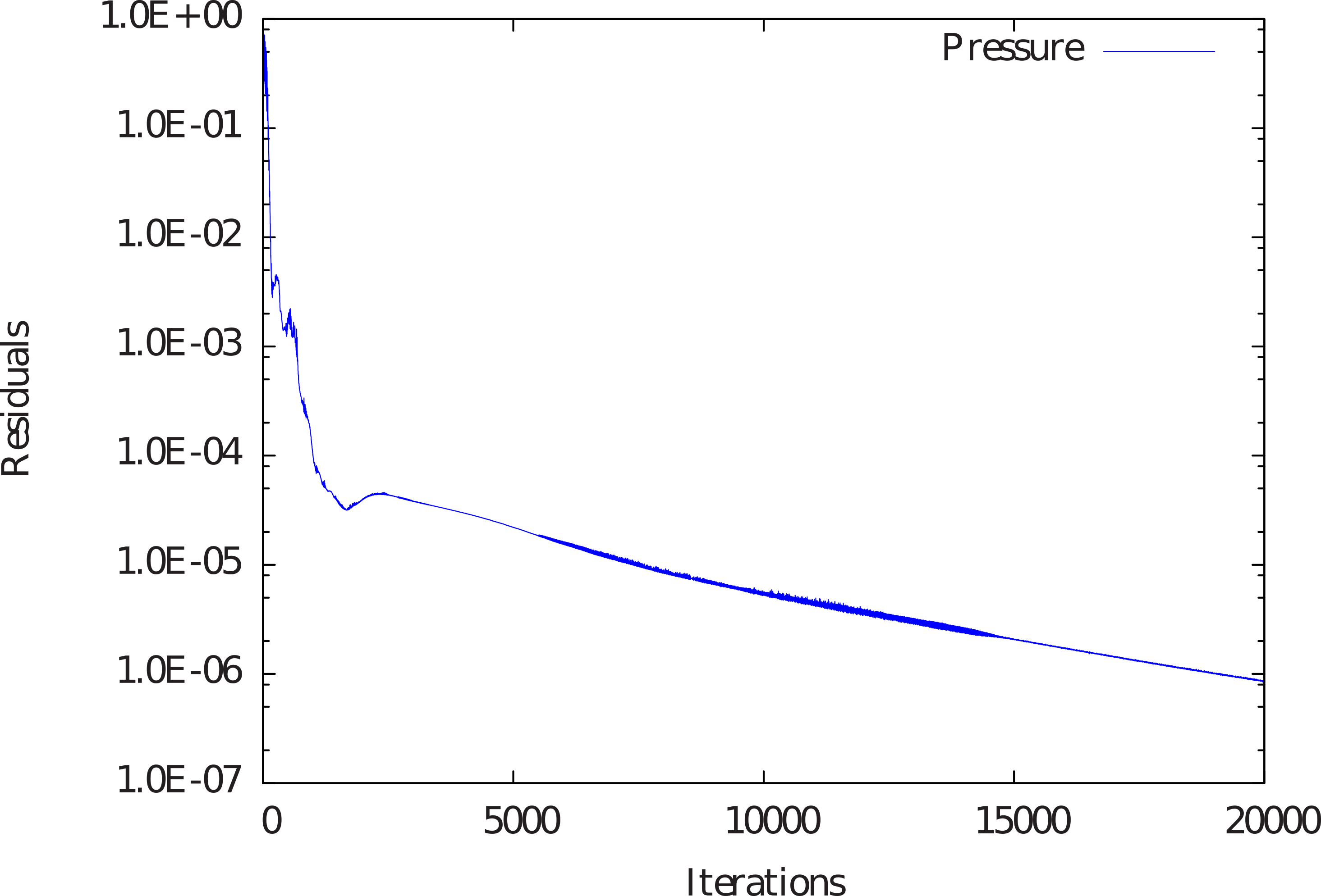
Figure 34 Convergence of pressure with respect to iterations
Results
The flow visualisation over the bump is shown here through the contours of velocity and pressure for SA model. In Figure 35 the variation of velocity and pressure can be seen as the bump is approached. As expected due to the curvature, flow accelerates while pressure reduces over the bump.
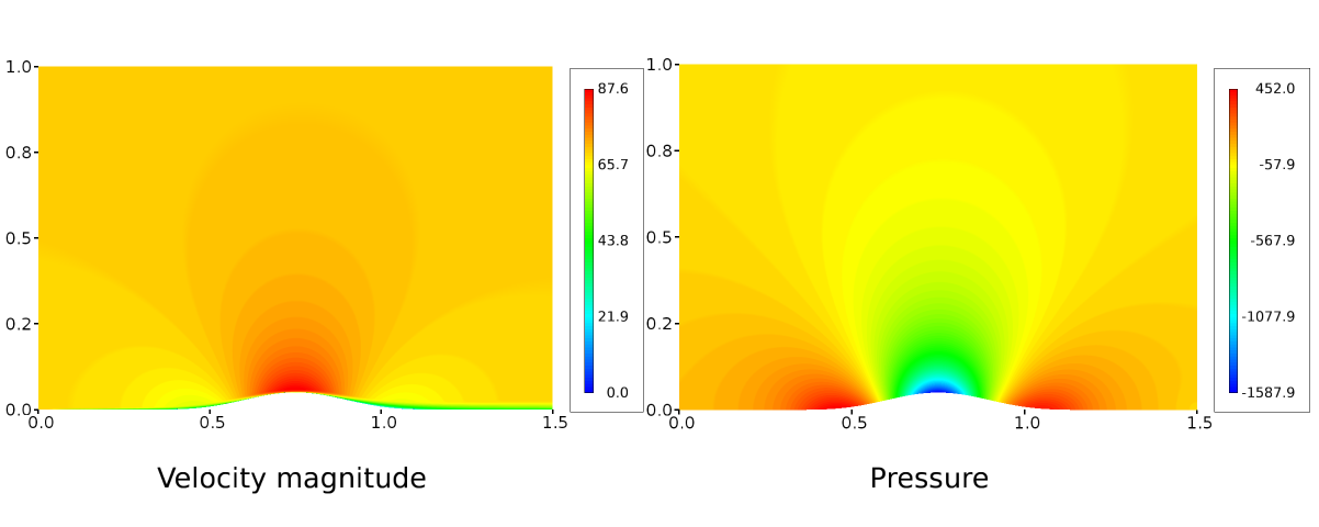
Figure 35 Contours of velocity and pressure over the bump surface
NACA Airfoil
In this tutorial, the turbulent flow over a two-dimensional NACA 0012 airfoil at two angles of attack, namely \(0^\circ\) and \(10^\circ\) will be considered. Caelus 9.04 will be used and the basic steps to set-up the directory structure, fluid properties, boundary conditions, turbulence properties etc will be shown. Visualisation of pressure and velocity over the airfoil are also shown. With these, the user should be able to reproduce the tutorial accurately.
Objectives
The user will get familiar in setting up Caelus simulation for steady, turbulent, incompressible flow over a two-dimensional airfoils at different angles of attack. Alongside, the user will be able to decompose the mesh on several CPUs performing a parallel simulation. Some of the steps that would be detailed are as follows
- Background
A brief description about the problem
Geometry and freestream details
- Grid generation
Computational domain and boundary details
Computational grid generation
Exporting grid to Caelus
- Problem definition
Directory structure
Setting up boundary conditions, physical properties and control/solver attributes
- Execution of the solver
Monitoring the convergence
Writing the log files
- Results
Visualisation of flow over the airfoil
Pre-requisites
It is understood that the user will be familiar with the Linux command line environment via a terminal or Caelus-console (For Windows OS) and Caelus is installed corrected with appropriate environment variables set. The grid for this case is obtained from Turbulence Modeling Resource as a Plot3D format and is converted to Caelus using Pointwise. The user is however free to use their choice of grid generation tool to convert the original Plot3D grid to Caelus readable format.
Background
Turbulent flow over airfoils is an interesting example to highlight some of the capabilities of Caelus. Here, the flow undergoes rapid expansion due to strong surface curvatures thereby inducing pressure and velocity gradients along the surface. Depending on shape of the curvature, adverse or favourable pressure gradients can exist on either side. These can be examined through surface quantities like pressure and skin-friction distributions. The user can refer to the verification and validation of this case at Two-dimensional NACA 0012 Airfoil.
The schematic of NACA 0012 airfoil at two angles of attack are shown in Figure 36 for a two-dimensional profile. A chord length (C) of 1.0 m is considered for both and has a Reynolds number of \(6 \times 10^6\). The flow is assumed to be Air with a freestream temperature of 300 K. Considering these values, the freestream velocity can be evaluated to U = 52.077 m/s. Note that the geometric plane considered for two-dimensionality is in \(x-z\) directions.
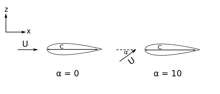
Figure 36 Schematic representation of the airfoil
The freestream conditions are given in the below table
Fluid |
\(C~(m)\) |
\(Re/L~(1/m)\) |
\(U~(m/s)\) |
\(p~(m^2/s^2)\) |
\(T~(K)\) |
\(\nu~(m^2/s)\) |
|---|---|---|---|---|---|---|
Air |
1.0 |
\(6 \times 10^6\) |
52.0770 |
Gauge (0) |
300 |
\(8.6795\times10^{-6}\) |
As noted earlier, flow at two angles of attack (\(\alpha\)) will be considered in this tutorial. In order to obtain a free-stream velocity of 52.0770 m/s at \(\alpha = 0^\circ\) and \(10^\circ\), the velocity components in \(x\) and \(z\) have to be resolved. The following table provides these values
\(\alpha~\rm{Degrees}\) |
\(u~(m/s)\) |
\(w~(m/s)\) |
|---|---|---|
\(0^\circ\) |
52.0770 |
0.0 |
\(10^\circ\) |
51.2858 |
9.04307 |
Grid Generation
The structured grid used for this tutorial can cells obtained from Turbulence Modeling Resource in Plot3D format that contains 512 around the airfoil and 256 cells in the flow normal direction. This should be then converted to polyMesh format.
The computational domain for the NACA 0012 airfoil is shown in Figure 37 along with the boundary conditions. A large domain exists around the airfoil (highlighted in blue) extending 500 chord lengths in the radial direction and the inlet condition is given for the entire boundary highlighted in green, whereas the outlet is placed at the exit plane which is about \(x \approx 500~m\). The velocity on the airfoil surface is zero, wherein \(u, v, w = 0\) represented through a no-slip boundary.
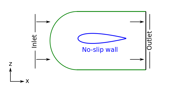
Figure 37 Computational domain of a 2D airfoil
The polyMesh grid is in three-dimensions, however the flow over airfoils can be assumed to be 2D at low angles of attack and is solved here in \(x-z\) directions. Therefore, a one-cell thick grid normal to the 2D flow plane is sufficient, where the flow can be assumed to be symmetry. The two \(x-z\) planes that are prevalent require boundary conditions to be specified. Since the flow is assumed to be 2D, we do not need to solve the flow in the third-dimension and this can be easily achieved in Caelus by specifying empty boundary conditions for each of the two planes. Consequently, the flow will be treated as symmetry in \(y\) direction.
Note
A velocity value of \(v=0\) needs to be specified at appropriate boundaries although no flow is solved in the \(y\) direction.
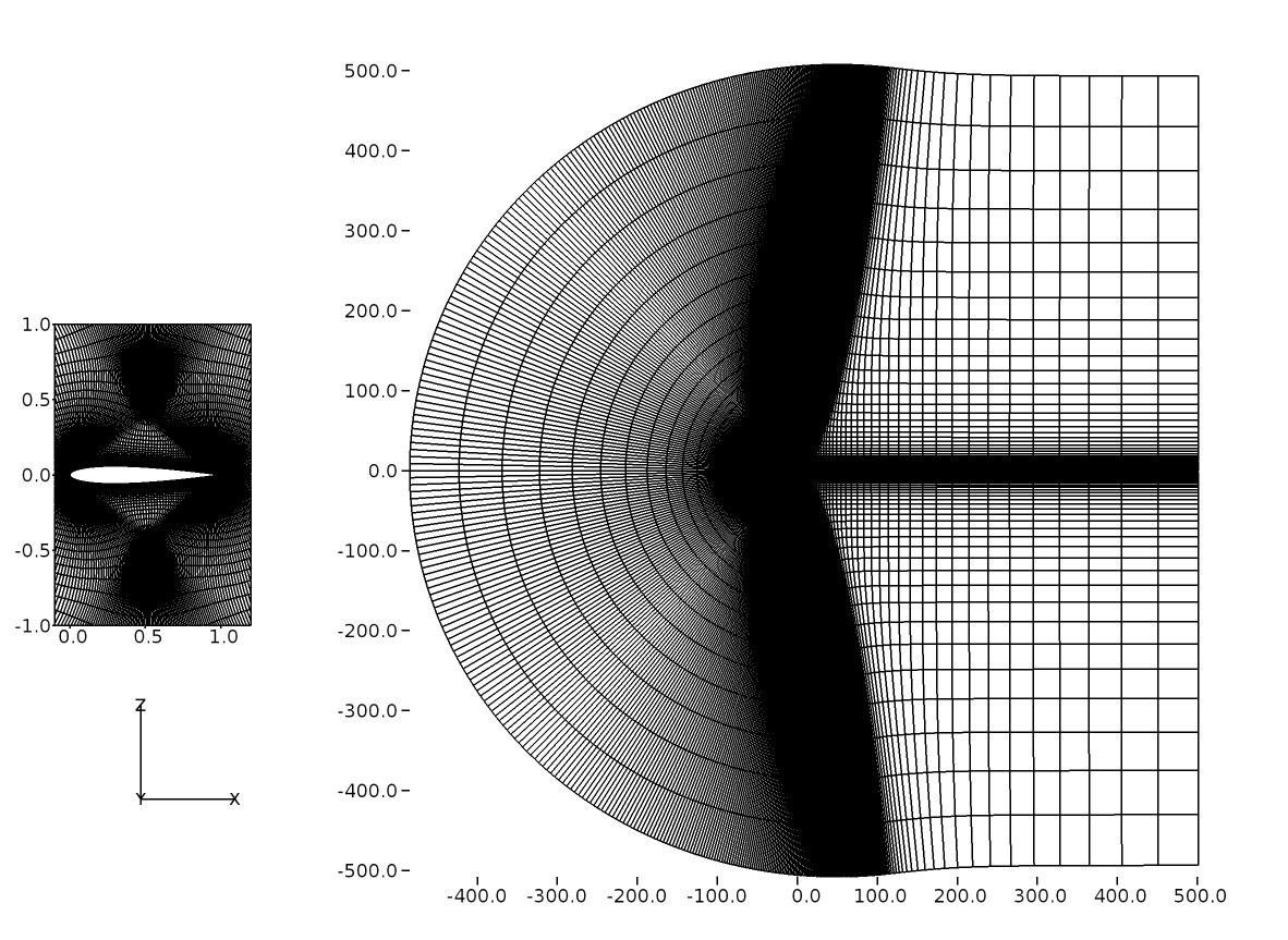
Figure 38 Computational grid of a 2D airfoil in \(x-z\) plane
The 2D airfoil grid in \(x-z\) plane is shown in Figure 38 which has a distribution of 512 X 256 cells. The grid in the vicinity of airfoil is shown as an inset and a very fine distribution can be noted very close to the wall. It was estimated that \(y^+\) is less than 1 to capture the turbulent boundary layer accurately and no wall-function is used.
Problem definition
In this section, various steps needed to set-up the turbulent flow over an airfoil will be shown. A full working case of this can be found in:
/tutorials/incompressible/simpleSolver/ras/ACCM_airFoil2D
However,the user is free to start the case setup from scratch consistent with the directory stucture discussed below.
Directory Structure
Note
All commands shown here are entered in a terminal window, unless otherwise mentioned
The problem requires time, constant and system sub-directories within the main working directory. Here, the simulation will be started at time t = 0 s, which requires a time sub-directory named 0.
The 0 sub-directory has files in which boundary properties are specified. In the below table, the list of necessary files are provided based on the turbulence model chosen
Parameter |
File name |
|---|---|
Pressure (\(p\)) |
|
Velocity (\(U\)) |
|
Turbulent viscosity (\(\nu\)) |
|
Turbulence field variable (\(\tilde{\nu}\)) |
|
Turbulent kinetic energy (\(k\)) |
|
Turbulent dissipation rate (\(\omega\)) |
|
We will consider two turbulence models in this tutorial, namely Spalart-Allmaras (SA) and \(k-\omega\) - Shear Stress Transport (\(\rm{SST}\)). The contents of the files listed above sets the dimensions, initialisation and boundary conditions to the defining problem, which also forms three principle entries required.
The user should note that Caelus is case sensitive and therefore the directory and file set-up should be identical to what is shown here.
Boundary Conditions and Solver Attributes
Boundary Conditions
Referring back to Figure 37, the following are the boundary conditions that will be specified:
- Inlet
Velocity:
\(\alpha=0^\circ\): Fixed uniform velocity \(u = 52.0770~m/s\); \(v = w = 0.0~m/s\) in \(x, y\) and \(z\) directions respectively
\(\alpha=10^\circ\): Fixed uniform velocity \(u = 51.2858~m/s\); \(v = 0.0~m/s\) and \(w = 9.04307~m/s\) in \(x, y\) and \(z\) directions respectively
Pressure: Zero gradient
Turbulence:
Spalart–Allmaras (Fixed uniform values of \(\nu_{t~\infty}\) and \(\tilde{\nu}_{\infty}\) as given in Turbulent freestream conditions for SA Model)
\(k-\omega~\rm{SST}\) (Fixed uniform values of \(k_{\infty}\), \(\omega_{\infty}\) and \(\nu_{t~\infty}\) as given in Turbulent freestream conditions for SST Model)
- No-slip wall
Velocity: Fixed uniform velocity \(u, v, w = 0\)
Pressure: Zero gradient
Turbulence:
Spalart–Allmaras (Fixed unifSpalart–Allmaras (Fixed uniform values of \(\nu_{t}=0\) and \(\tilde{\nu}=0\))
\(k-\omega~\rm{SST}\) (Fixed uniform values of \(k = <<0\) and \(\nu_t=0\); \(\omega\) = omegaWallFunction)
- Outlet
Velocity: Zero gradient velocity
Pressure: Fixed uniform gauge pressure \(p = 0\)
Turbulence:
Spalart–Allmaras (Calculated \(\nu_{t}=0\) and Zero gradient \(\tilde{\nu}\))
\(k-\omega~\rm{SST}\) (Zero gradient \(k\) and \(\omega\); Calculated \(\nu_t=0\); )
- Initialisation
Velocity:
\(\alpha=0^\circ\): Fixed uniform velocity \(u = 52.0770~m/s\); \(v = w = 0.0~m/s\) in \(x, y\) and \(z\) directions respectively
\(\alpha=10^\circ\): Fixed uniform velocity \(u = 51.2858~m/s\); \(v = 0.0~m/s\) and \(w = 9.04307~m/s\) in \(x, y\) and \(z\) directions
Pressure: Zero Gauge pressure
Turbulence:
Spalart–Allmaras (Fixed uniform values of \(\nu_{t~\infty}\) and \(\tilde{\nu}_{\infty}\) as given in Turbulent freestream conditions for SA Model)
\(k-\omega~\rm{SST}\) (Fixed uniform values of \(k_{\infty}\), \(\omega_{\infty}\) and \(\nu_{t~\infty}\) as given in Turbulent freestream conditions for SST Model)
First, the pressure file named p has the following contents
/*---------------------------------------------------------------------------*\
Caelus 9.04
 Web:      www.caelus-cml.com
\*---------------------------------------------------------------------------*/
FoamFile
{
    version     2.0;
    format      ascii;
    class       volScalarField;
    location    "0";
    object      p;
}
// * * * * * * * * * * * * * * * * * * * * * * * * * * * * * * * * * * * * * //

dimensions      [0 2 -2 0 0 0 0];

internalField   uniform 0;

boundaryField
{
    inlet
    {
        type            zeroGradient;
    }
    left
    {
        type            empty;
    }
    outlet
    {
        type            fixedValue;
        value           uniform 0;
    }
    right
    {
        type            empty;
    }
    wall
    {
        type            zeroGradient;
    }
}


// ************************************************************************* //
In the information shown above, it can be seen that the file begins with a dictionary named FoamFile which contains the standard set of keywords for version, format, location, class and object names. The explanation of the principle entries are as follows
dimensionis used to specify the physical dimensions of the pressure field. Here, pressure is defined in terms of kinematic pressure with the units (\(m^2/s^2\)) written as
[0 2 -2 0 0 0 0]
internalFieldis used to specify the initial conditions. It can be either uniform or non-uniform. Since we have a 0 initial uniform gauge pressure, the entry is
uniform 0;
boundaryFieldis used to specify the boundary conditions. In this case its the boundary conditions for pressure at all the boundary patches.
Similarly, the file U is defined as follows,
/*---------------------------------------------------------------------------*\
Caelus 9.04
 Web:      www.caelus-cml.com
\*---------------------------------------------------------------------------*/
FoamFile
{
    version     2.0;
    format      ascii;
    class       volVectorField;
    location    "0";
    object      U;
}
// * * * * * * * * * * * * * * * * * * * * * * * * * * * * * * * * * * * * * //

dimensions      [0 1 -1 0 0 0 0];

internalField   uniform (52.077 0 0);

boundaryField
{
    inlet
    {
        type            fixedValue;
        value           uniform (52.077 0 0);
    }
    left
    {
        type            empty;
    }
    outlet
    {
        type            zeroGradient;
    }
    right
    {
        type            empty;
    }
    wall
    {
        type            noSlipWall;
    }
}


// ************************************************************************* //
The principle entries for velocity field are self-explanatory and the dimensions are typically for that of velocity with the units \(m/s\) ([0 1 -1 0 0 0 0]). The user should note that appropriate entry has to be enabled for both internalField and inlet boundaryField depending on which angle of attack (AOA/\(\alpha\)) is being simulated. Here, both initialisation and inlet have a uniform flow velocity specified with three velocity components. For example at \(\alpha = 10^\circ\), we specify (51.2858 0 9.04307) for \(u, v, w\) components respectively. Similarly, the wall boundary patch have three velocity components.
The turbulent properties are also required to be specified at the boundary patches and these can be done similar to p and U. The file nut, defines turbulent kinematic viscosity and its boundary conditions as follows.
/*---------------------------------------------------------------------------*\
Caelus 9.04
 Web:      www.caelus-cml.com
\*---------------------------------------------------------------------------*/
FoamFile
{
    version     2.0;
    format      ascii;
    class       volScalarField;
    location    "0";
    object      nut;
}
// * * * * * * * * * * * * * * * * * * * * * * * * * * * * * * * * * * * * * //

dimensions      [0 2 -1 0 0 0 0];

internalField   uniform 1.8265e-06;

boundaryField
{
    inlet
    {
        type            fixedValue;
        value           uniform 1.8265e-06;
    }
    left
    {
        type            empty;
    }
    outlet
    {
        type            calculated;
        value           uniform 0;
    }
    right
    {
        type            empty;
    }
    wall
    {
        type            fixedValue;
        value           uniform 0;
    }
}


// ************************************************************************* //
As noted above, the turbulent viscosity is specified as kinematic and therefore the units are in \(m^2/s\) ([0 2 -1 0 0 0 0]). The turbulent viscosity value at freestream, specified at inlet patch is calculated as detailed in Turbulent freestream conditions for SA Model and Turbulent freestream conditions for SST Model for SA and SST models respectively and is specified accordingly. The same value also goes for internalField. Note that a fixedValue of 0 is used for the wall which suggests that on the wall, it is only the molecular (laminar) viscosity that prevails.
The next turbulent property to set is the nuTilda which is a turbulent field variable, specified to only SA model and has the same units ([0 2 -1 0 0 0 0]) as kinematic turbulent viscosity. Details pertaining to this are given in Turbulent freestream conditions for SA Model. The following are the contents of the file nuTilda and the entries specified for the boundaryField are identical to that of turbulent kinematic viscosity explained above.
/*---------------------------------------------------------------------------*\
Caelus 9.04
 Web:      www.caelus-cml.com
\*---------------------------------------------------------------------------*/
FoamFile
{
    version     2.0;
    format      ascii;
    class       volScalarField;
    location    "0";
    object      nuTilda;
}
// * * * * * * * * * * * * * * * * * * * * * * * * * * * * * * * * * * * * * //

dimensions      [0 2 -1 0 0 0 0];

internalField   uniform 2.60385e-05;

boundaryField
{
    inlet
    {
        type            fixedValue;
        value           uniform 2.60385e-05;
    }
    left
    {
        type            empty;
    }
    outlet
    {
        type            zeroGradient;
    }
    right
    {
        type            empty;
    }
    wall
    {
        type            fixedValue;
        value           uniform 0;
    }
}


// ************************************************************************* //
We can now proceed to the files k and omega, specific to only \(k-\omega~\rm{SST}\) model. \(k-\omega~\rm{SST}\) is a turbulence model which solves for turbulent kinetic energy and the specific rate of dissipation using two partial differential equations. Caelus therefore requires information about these to be specified at the boundary patches when this model is chosen. Starting with the file k,
/*---------------------------------------------------------------------------*\
Caelus 9.04
 Web:      www.caelus-cml.com
\*---------------------------------------------------------------------------*/
FoamFile
{
    version     2.0;
    format      ascii;
    class       volScalarField;
    location    "0";
    object      k;
}
// * * * * * * * * * * * * * * * * * * * * * * * * * * * * * * * * * * * * * //

dimensions      [0 2 -2 0 0 0 0];

internalField   uniform 0.0010999;

boundaryField
{
    inlet
    {
        type            fixedValue;
        value           uniform 0.0010999;
    }
    left
    {
        type            empty;
    }
    outlet
    {
        type            zeroGradient;
    }
    right
    {
        type            empty;
    }
    wall
    {
        type            fixedValue;
        value           uniform 1e-10;
    }
}


// ************************************************************************* //
The unit of kinetic energy is \(m^2/s^2\) and this is set in dimensions as [0 2 -2 0 0 0 0]. As with other turbulent quantities discussed above, the value of \(k\) (refer Turbulent freestream conditions for SST Model) needs to be specified for internalField, inlet and wall. Please note that for wall boundaryField with no wall-function, a small, non-zero fixedValue is required.
We now proceed to the file omega and the value for this is evaluated as detailed in Turbulent freestream conditions for SST Model
/*---------------------------------------------------------------------------*\
Caelus 9.04
 Web:      www.caelus-cml.com
\*---------------------------------------------------------------------------*/
FoamFile
{
    version     2.0;
    format      ascii;
    class       volScalarField;
    location    "0";
    object      omega;
}
// * * * * * * * * * * * * * * * * * * * * * * * * * * * * * * * * * * * * * //

dimensions      [0 0 -1 0 0 0 0];

internalField   uniform 13887.21912;

boundaryField
{
    inlet
    {
        type            fixedValue;
        value           uniform 13887.21912;
    }
    left
    {
        type            empty;
    }
    outlet
    {
        type            zeroGradient;
    }
    right
    {
        type            empty;
    }
    wall
    {
        type            omegaWallFunction;
        value           uniform 1;
    }
}


// ************************************************************************* //
The unit of specific rate of dissipation for \(\omega\) is \(1/s\) which is set in dimensions as [0 0 -1 0 0 0 0]. The internalField and inlet gets a fixedValue. Note that for wall boundaryField, we specify omegaWallFunction and this is a model requirement and sets omega to the correct value near wall based on the \(y^+\). In conjunction, the value that goes with omegaWallFunction can be anything and for simplicity its set to 1.
Before proceeding to the next step, it is vital to ensure that the boundary conditions (inlet, outlet, wall, etc) added in the above files should be the grid boundary patches (surfaces) generated by grid generation tool and their names are identical. Additionally, the two boundaries \(x-z\) plane named here as left and right have empty boundary conditions which forces Caelus to assume the flow to be in two-dimensions. With this, the setting up of the boundary conditions are complete.
Grid file and Physical Properties
The grid files associated with the NACA airfoil need to be placed in polyMesh sub-directory, which resides in the constant directory. Note that for both angles of attack, the identical grid is used. This is because the flow incidence angle is relative to the fixed airfoil and the equivalent velocity components can be easily specified thus simulating the airfoil at the required angle of attack. In addition, the physical properties are specified in various different files present in the constant directory.
polyMesh RASProperties transportProperties turbulenceProperties
As seen above, the three files are listed in addition to the polyMesh sub-directory. The first one, RASProperties in which the Reynolds-Average-Stress (RAS) model is specified, which is shown below. Please note that depending on the turbulence model you wish to run with, the line that corresponds to that specific model should be enabled.
/*-------------------------------------------------------------------------------*
Caelus 9.04
Web:   www.caelus-cml.com
\*------------------------------------------------------------------------------*/

FoamFile
{
	version				2.0;
	format				ascii;
	class				dictionary;
	location			"constant";
	object				RASProperties;
}

//--------------------------------------------------------------------------------

// For Spalarat-Alamaras Model, enable the below line
RASModel				SpalartAllmaras;

// For k-omega SST Model, enable the below line
// RASModel				kOmegaSST;

turbulence				on;

printCoeffs				on;

SpalartAllmarasCoeffs
{
    curvatureCorrection off;
}

kOmegaSSTCoeffs
{
    curvatureCorrection off;
    Cscale          1;
    frMax           1.25;
}
Second from the list is the transportProperties file, where kinematic viscosity is specified as shown below
/*-------------------------------------------------------------------------------*
Caelus 9.04
Web:   www.caelus-cml.com
\*------------------------------------------------------------------------------*/

FoamFile
{
	version				2.0;
	format				ascii;
	class				dictionary;
	location			"constant";
	object				transportProperties;
}

//--------------------------------------------------------------------------------

transportModel				Newtonian;

nu					nu [0 2 -1 0 0 0 0] 8.679514E-6;
The viscous behaviour is modelled as Newtonian and hence the keyword Newtonian is used for the transportModel and the molecular (laminar) kinematic viscosity (\(nu\)) is given having the units \(m^2/s\) ([0 2 -1 0 0 0 0]).
The final file in this class is the turbulenceProperties file, which sets the simulationType to RASModel. Both SA and \(k-\omega~\rm{SST}\) are classified as Reynolds Average Stress (RAS) models.
/*-------------------------------------------------------------------------------*
Caelus 9.04
Web:   www.caelus-cml.com
\*------------------------------------------------------------------------------*/

FoamFile
{
	version				2.0;
	format				ascii;
	class				dictionary;
	location			"constant";
	object				turbulenceProperties;
}

//--------------------------------------------------------------------------------

simulationType				RASModel;
Controls and Solver Attributes
In this section, the files required to control the simulation, specifying discretisation methods and linear solver settings are given. These files are to be placed in the system directory. First, navigate to the system directory.
The controlDict file contains the following details
/*-------------------------------------------------------------------------------*
Caelus 9.04
Web:   www.caelus-cml.com
\*------------------------------------------------------------------------------*/
FoamFile
{
   version          2.0;
   format           ascii;
   class            dictionary;
   location         "system";
   object           controlDict;
}
//-------------------------------------------------------------------------------

application         simpleSolver;

startFrom           startTime;

startTime           0;

stopAt              endTime;

endTime             10000; // increase endTime to atleast 50000 for validation cases

deltaT              1;

writeControl        runTime;

writeInterval       1000;

purgeWrite          2;

writeFormat         ascii;

writePrecision      12;

writeCompression    true;

timeFormat          general;

timePrecision       6;

runTimeModifiable   true;

//-------------------------------------------------------------------------------

// Function Objects to obtain forces

functions
{
    forces
    {
        type            forces;

        functionObjectLibs ("libforces.so");
        patches         ( wall );
        CofR            (0 0 0);
        rhoName         rhoInf;
        rhoInf          2.15527;
        writeControl    timeStep;
        writeInterval   50;
    }
}
Referring to the above file, some explanation is required. Here, simpleSolver is used and the simulation begins at t = 0 s. This now explains the logical need for having a 0 directory where the data files are read at the beginning of the run, which is t = 0 s in this case. Therefore, the keyword startFrom is set to startTime, where startTime is set to 0. The simulation would be carried out as steady-state and therefore we require to specify the total number of iterations as a keyword for endTime. Via the writeControl and writeInterval keywords, the solution intervals at which they are saved can be specified. Also note that a function object to obtain the force over the wall (airfoil surface) for every 50 iterations is included. In order to obtain this, a freestream density (rhoInf) need to be specified.
The discretization schemes for the finite volume discretization that will be used should be set through the fvSchemes file shown below.
/*-------------------------------------------------------------------------------*
Caelus 9.04
Web:   www.caelus-cml.com
\*------------------------------------------------------------------------------*/
FoamFile
{
    version         2.0;
    format          ascii;
    class           dictionary;
    object          fvSchemes;
}
//------------------------------------------------------------------------------

ddtSchemes
{
   default              steadyState;
}

gradSchemes
{
   default              Gauss linear;
}

divSchemes
{
   default              none;
   div(phi,U)           Gauss linearUpwindBJ grad(U);
   div(phi,nuTilda)     Gauss upwind;
   div(phi,k)           Gauss upwind;
   div(phi,omega)       Gauss upwind;
   div((nuEff*dev(T(grad(U))))) Gauss linear;
   div(phi,symm(grad(U))) Gauss linear;
}

laplacianSchemes
{
   default              none;
   laplacian(nu,U)      Gauss linear corrected;
   laplacian(nuEff,U)   Gauss linear corrected;
   laplacian(DnuTildaEff,nuTilda) Gauss linear corrected;
   laplacian(DkEff,k) Gauss linear corrected;
   laplacian(DomegaEff,omega) Gauss linear corrected;
   laplacian(rAUf,p)    Gauss linear corrected;
   laplacian(1,p)       Gauss linear corrected;
}

interpolationSchemes
{
   default              linear;
   interpolate(HbyA)    linear;
}

snGradschemes
{
   default              corrected;
}
The linear solver controls and tolerances are set in fvSolution as given below
/*-------------------------------------------------------------------------------*
Caelus 9.04
Web:   www.caelus-cml.com
\*------------------------------------------------------------------------------*/
FoamFile
{
        version                         2.0;
        format                          ascii;
        class                           dictionary;
        location                        "system";
        object                          fvSolution;
}
//------------------------------------------------------------------------------

solvers
{
    p
    {
        solver                  PCG;
        preconditioner
        {
            preconditioner          GAMG;
            smoother                SSGS;
            cacheAgglomeration      true;
            nCellsInCoarsestLevel   10;
            agglomerator            algebraicPair;
            mergeLevels             1;
        }

        tolerance               1e-16;
        relTol                  0.01;
    }

    U
    {
        solver                  PBiCGStab;
        preconditioner          USGS;
        tolerance               1e-16;
        relTol                  0.1;
    }

    "(k|omega|nuTilda)"
    {
        solver                  PBiCGStab;
        preconditioner          USGS;
        tolerance               1e-16;
        relTol                  0.1;
    }
}

SIMPLE
{
    nNonOrthogonalCorrectors    1;
    pRefCell                    0;
    pRefValue                   0;
    consistent                  yes;
    correctionFoam              yes;
}

// relexation factors

relaxationFactors
{
    p                           0.3;
    U                           0.7;
    nuTilda                     0.7;
    k                           0.7;
    omega                       0.7;
}
The user should now take a note that in the fvSolution file, different linear solvers are used to solve for velocity, pressure and turbulence quantities We also set the nNonOrthogonalCorrectors to 1 for this case. To ensure the stability of the solution, the relaxation is set to primary and turbulent variables. The relTol is not set to 0 unlike a time-accurate set-up as we are solving for a steady-state solution and a very low (\(\approx 0\)) tolerance at every iteration is unnecessary. Since the entire system of equations converge to a global set tolerance the convergence would occur as the solution progresses to a steady state.
With this, the set-up of the directory structure with all the relevant files are complete. This can be verified again by issuing the following command and the directory tree should appear identical to the one shown below
cd my-turbulent-airfoil/
tree
.
├── 0
│   ├── epsilon
│   ├── k
│   ├── nut
│   ├── nuTilda
│   ├── omega
│   ├── p
│   └── U
├── constant
│   ├── polyMesh
│   │   ├── boundary
│   │   ├── faces
│   │   ├── neighbour
│   │   ├── owner
│   │   └── points
│   ├── RASProperties
│   ├── transportProperties
│   └── turbulenceProperties
└── system
    ├── controlDict
    ├── decomposePar
    ├── fvSchemes
    └── fvSolution
Execution of the solver
Before executing the solver, it is important to renumber and to carry out a quality check on the grid/mesh. Renumbering reduces the bandwidth whereas the quality check shows the mesh statistics. These two can be performed by executing the following commands from the top working directory
caelus run -- renumberMesh -overwrite
caelus run -- checkMesh
When the renumberMesh is performed, the user should take note of the bandwidth before and after the mesh renumbering. In a similar manner, when the checkMesh is performed, the mesh statistics are shown as below
/*---------------------------------------------------------------------------*\
 Caelus 8.04
 Web:      www.caelus-cml.com
\*---------------------------------------------------------------------------*/

Checking geometry...
    Overall domain bounding box (-484.456616748 0 -507.806809185) (501.000007802 10 507.806808887)
    Mesh (non-empty, non-wedge) directions (1 0 1)
    Mesh (non-empty) directions (1 0 1)
    All edges aligned with or perpendicular to non-empty directions.
    Boundary openness (8.28364670182e-18 1.55457412622e-15 -1.3301799376e-17) OK.
 ***High aspect ratio cells found, Max aspect ratio: 31784747.6728, number of cells 29164
  <<Writing 29164 cells with high aspect ratio to set highAspectRatioCells
    Minimum face area = 9.57960157047e-11. Maximum face area = 843.777295738.  Face area magnitudes OK.
    Min volume = 9.57960157047e-10. Max volume = 8437.77295738.  Total volume = 8755584.35466.  Cell volumes OK.
    Mesh non-orthogonality Max: 57.3127287926 average: 1.73980453241
    Non-orthogonality check OK.
    Face pyramids OK.
    Mesh skewness Max: 0.201755632336 average: 0.00254964789178 OK.
    Coupled point location match (average 0) OK.

Failed 1 mesh checks.

End
As can be noted above, the output of the checkMesh indicates that the mesh check has failed reporting in the final message as Failed 1 mesh checks. This is because of the high aspect ratio meshes present immediate to the wall with very low (\(<< y^+\)) values. Nevertheless, this is just a warning and Caelus will solve on this mesh.
As with the previous tutorial, it will be shown here to utilise the multi-core capability of CPUs for performing a parallel computation using MPI technique for large grids, such as the one considered here. Before this can be done, the grid has to be decomposed into smaller domains that can be solved by each single CPU core. The number of decomposition should be equal to the number of CPU core available for parallel computing. The decomposition is carried out through a file decomposeParDict present in the system sub-directory as shown below.
/*-------------------------------------------------------------------------------*
Caelus 9.04
Web:   www.caelus-cml.com
\*------------------------------------------------------------------------------*/

FoamFile
{
    version     		2.0;
    format      		ascii;
    class       		dictionary;
    object      		decomposeParDict;
}
//--------------------------------------------------------------------------------

numberOfSubdomains 		4; // It is suggested that the numberOfSubdomains be increased based on available resources for validation cases and to reduce the computation time.

method          		scotch;

distributed     		no;

roots
(
);
In the above file, the the keyword numberOfSubdomains defines the number of decomposed sub-domains needed and 4 is used which partitions the grid into 4 sub-domains. We use scotch as the method of decomposition which automatically divides the gird. The execution to decompose the grid is carried out again from the top directory as follows
caelus run -- decomposePar
Now the decomposition should begin and the details of which are displayed in the terminal window. Subsequently, 4 processor directories will be generated as we have requested for 4 divisions of grid as shown below
0 constant processor0 processor1 processor2 processor3 system
The solver can now be executed for parallel computation in the host machine from the top directory using the following command
caelus run -p -l my-turbulent-airfoil.log -- simpleSolver
Note that here it is assumed that the parallel computing is available in the host machine. With the execution of the above commands, the simulation begins and the progress of the solution is written to the specified log file (my-turbulent-airfoil.log).
The log file can be further processed to look at the convergence history and this can be done as follows
caelus logs -w my-turbulent-airfoil.log
The above command allows you to look at the convergence of different variables with respect to the number of iterations carried out. The convergence of pressure is shown in Figure 39.
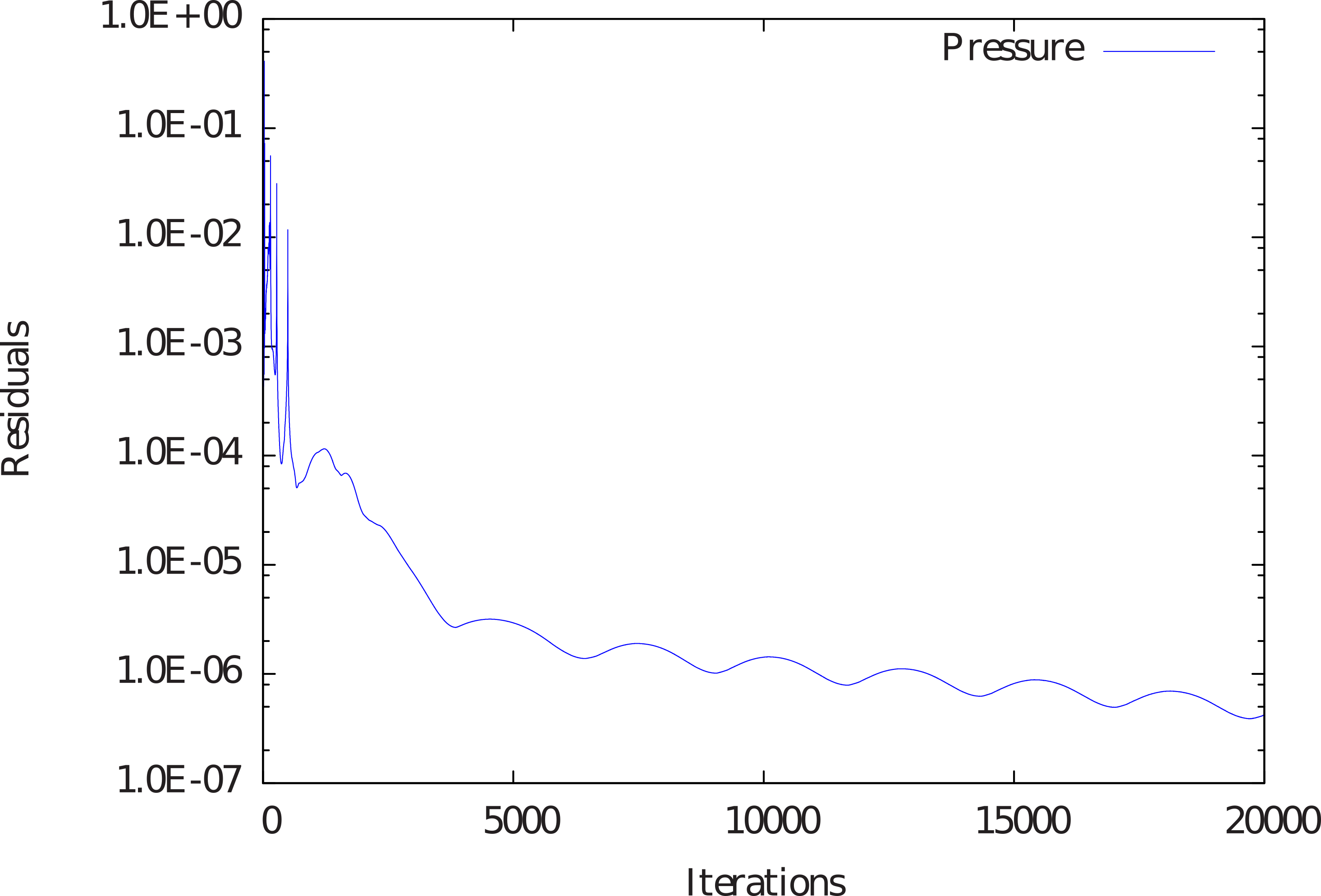
Figure 39 Convergence of pressure with respect to iterations
Results
The flow over the airfoil at both \(0^\circ\) and \(10^\circ\) degree angle of attack are presented here. In Figure 40, velocity magnitude and pressure contours can be seen for \(\alpha = 0^\circ\) angle of attack. These result are for the SA model. The suction and the pressure surfaces essentially produce the same flow due to \(0^\circ\) angle of incidence and thus contributes to zero lift. In contrast, at \(0^\circ\) angle of incidence in Figure 41, a low pressure region exists on the upper surface and consequently the velocity increases thus generating some lift.
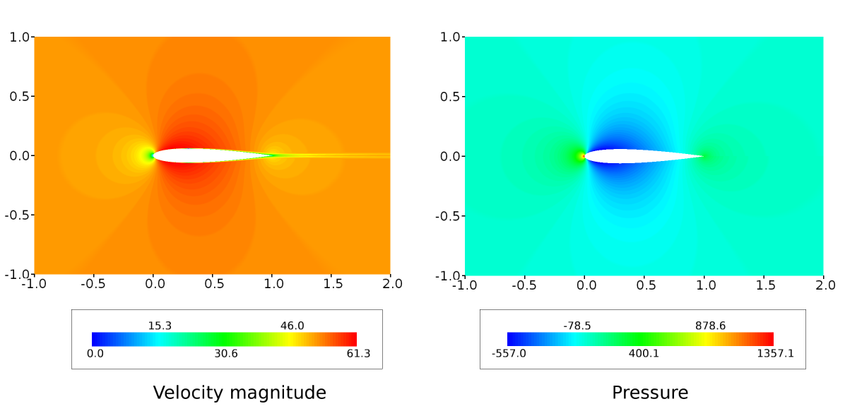
Figure 40 Velocity magnitude and pressure contours for \(\alpha = 0^\circ\) angle of attack
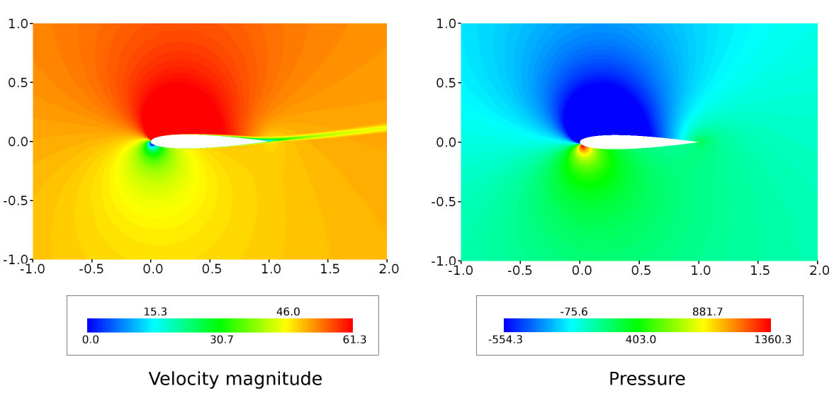
Figure 41 Velocity magnitude and pressure contours for \(\alpha = 10^\circ\) angle of attack
Convex Curvature
Turbulent flow in a constant-area duct having a convex curvature is considered in this tutorial. Caelus 9.04 will be used and the process of setting-up of directory structure, fluid properties, boundary conditions, turbulent properties, etc will be explained here. In addition to this, the flow within the duct will be visualised. The steps would be sufficient for the user to reproduce the tutorial accurately.
Objectives
Through this tutorial, the user will get familiarise with setting up the Caelus simulation for steady, turbulent, incompressible flow in a two-dimensional duct having a convex curvature and subsequently post-process the results. The steps that would be followed in this tutorial is outlined below
- Background
A brief description about the problem
Geometry and inflow details
- Grid generation
Computational domain and boundary details
Computational grid generation
Exporting grid to Caelus
- Problem definition
Directory structure
Setting up boundary conditions, physical properties and control/solver attributes
- Execution of the solver
Monitoring the convergence
Writing the log files
- Results
Visualising the flow within the convex duct
Pre-requisites
It will be assumed that the user is comfortable and familiar with the Linux command line environment using a terminal or Caelus-console (on Windows OS). The user should also make sure that Caelus is installed correctly with appropriate environment variables set. The grid used here is obtained from Turbulence Modeling Resource in Plot 3D format and is exported to Caelus using Pointwise. The user can use their choice of grid generation tool to convert Plot3D file to Caelus format.
Background
Turbulent flow in a constant-area duct with a curvature is an interesting case. Here as a result of a curvature, pressure gradients occur in the vicinity of the curvature having localised effect. The flow will be assumed as steady-state and incompressible. Non-dimensional shear-stress (skin-friction coefficient) will be used to show the influence of curvature on the flow. Validation and verification of this exercise is detailed in section Two-dimensional Convex Curvature and the user is suggested to refer for more information.
The inlet of the duct as can be seen from the schematic below in Figure 42 has an inclination of \(\alpha = 30^\circ\). This is followed by a rapid bend at the same angle, \(\alpha\) after a distance of about 1.4 m. The downstream extends to 1.6 meters. The inflow has a Reynolds number of \(2.1 \times 10^6\), with Air as the fluid. The temperature of the inflow is at 293 K and U is the inlet velocity. Based on the Reynolds number, temperature and velocity, the kinematic viscosity is evaluated to \(\nu = 1.519470 \times 10^{-5}~m^2/s\). The geometric-plane for this case in 2-D is \(x-z\) plane.
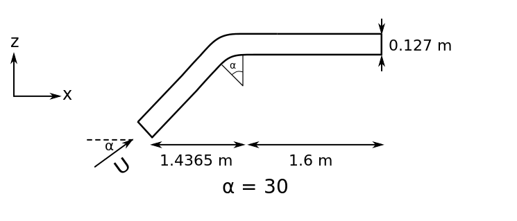
Figure 42 Schematic representation of the 2D curvature geometry
The inflow conditions for this case is given in the below table (Freestream conditions)
Fluid |
\(Re/L~(1/m)\) |
\(U~(m/s)\) |
\(p~(m^2/s^2)\) |
\(T~(K)\) |
\(\nu~(m^2/s)\) |
|---|---|---|---|---|---|
Air |
\(2.1 \times 10^6\) |
31.9088 |
Gauge (0) |
293 |
\(1.5194\times10^{-6}\) |
To achieve a inlet velocity of U = 31.9088 m/s at \(\alpha = 30^\circ\), the velocity components in \(x\) and \(z\) are resolved. These are given in the below table
\(\alpha\) |
\(u~(m/s)\) |
\(w~(m/s)\) |
|---|---|---|
\(30^\circ\) |
27.63313 |
15.95443 |
Grid Generation
The structured grid for this case has been obtained from from Turbulence Modeling Resource in a Plot3 format which contains 512 cells in streamwise direction and 192 in the flow normal direction. The Plot3D file has to be converted to polyMesh format.
In Figure 43, the computational domain can be seen which as expected follows the geometry. The velocity at the internal walls (highlighted in blue) are zero, wherein \(u, v, w =0\) representing a no-slip boundary. The inlet and the outlet are applied to the start and end of the domain respectively.
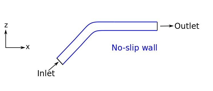
Figure 43 Computational domain of the convex curvature
The grid that is used, polyMesh format is in three-dimensions. However it is assumed that the flow through the duct can be modelled as 2D and is the 2D plane considered for this case is \(x-z\) directions. As with all the previous cases, one-cell thick normal to the 2D plane is sufficient, assuming the flow to be symmetry. The two \(x-z\) planes that are present in the grid require boundary conditions to be specified. An empty boundary condition can be used in Caelus for the two planes that forces the solver not to solve in the third-dimension, essentially treating the flow as symmetry in \(y\) direction.
Note
A velocity value of \(v=0\) needs to be specified at appropriate boundaries although no flow is solved in the \(y\) direction.
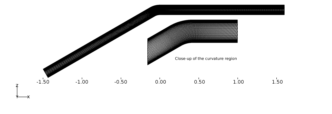
Figure 44 Convex curvature grid in two-dimensions in \(x-z\) plane
The 2D grid in \(x-z\) plane is shown in Figure 44 having a distribution of 512 X 192 cells. The inset in the figure highlights the region vicinity of the curvature and very fine distribution of cells can be seen close to the wall. It is estimated that \(y^+\) is less than 1 in order to capture turbulent boundary layer accurately and thus no wall-function is used.
Problem definition
This section details the various steps required to set-up the turbulent flow inside a convex duct. A full working case of this can be found in:
/tutorials/incompressible/simpleSolver/ras/ACCM_convexCurvature2D
Directory Structure
Note
All commands shown here are entered in a terminal window, unless otherwise mentioned
A few more sub-directories are needed in the top-level directory to set-up the case. Caelus requires time, constant and system sub-directories within the main my-turbulent-curvature working directory. Since we start the simulation at time, t =0 s, a time sub-directory named 0 is required. A
The 0 sub-directory cotains the files in which boundary properties are specified. In the below table, the list of necessary files are provided based on the turbulence model chosen
Parameter |
File name |
|---|---|
Pressure (\(p\)) |
|
Velocity (\(U\)) |
|
Turbulent viscosity (\(\nu\)) |
|
Turbulence field variable (\(\tilde{\nu}\)) |
|
Turbulent kinetic energy (\(k\)) |
|
Turbulent dissipation rate (\(\omega\)) |
|
We consider simulating this case with three turbulence models, namely Spalart-Allmaras (SA), Spalart–Allmaras Rotational/Curvature (SA-RC) and \(k-\omega\) - Shear Stress Transport (\(\rm{SST}\)). The contents that are entered in these files set the dimensions, initialisation and boundary conditions to the defining problem, which also form three principle entries required.
Caelus is case sensitive and therefore the user should carefully set-up the case as shown here if applicable.
Boundary Conditions and Solver Attributes
Boundary Conditions
Referring back to figure Computational domain of the convex curvature, following are the boundary conditions that will be specified:
- Inlet
Velocity: Fixed uniform velocity \(u = 27.63313~m/s\); \(v = 0.0~m/s\) and \(w = 15.95443~m/s\) in \(x, y\) and \(z\) directions respectively
Pressure: Zero gradient
Turbulence:
SA & SA-RC (Fixed uniform values of \(\nu_{t~i}\) and \(\tilde{\nu}_{i}\) as given in Turbulent freestream conditions for SA Model)
\(k-\omega~\rm{SST}\) (Fixed uniform values of \(k_{i}\), \(\omega_{i}\) and \(\nu_{t~i}\) as given in Turbulent freestream conditions for SST Model)
- No-slip wall
Velocity: Fixed uniform velocity \(u, v, w = 0\)
Pressure: Zero gradient
Turbulence:
SA & SA-RC (Fixed uniform values of \(\nu_{t}=0\) and \(\tilde{\nu} =0\))
\(k-\omega~\rm{SST}\) (Fixed uniform values of \(k = <<0\) and \(\nu_t=0\); \(\omega\) = omegaWallFunction)
- Outlet
Velocity: Zero gradient velocity
Pressure: Fixed uniform gauge pressure \(p = 0\)
Turbulence:
SA & SA-RC (Calculated \(\nu_{t}=0\) and Zero gradient \(\tilde{\nu}\))
\(k-\omega~\rm{SST}\) (Zero gradient \(k\) and \(\omega\); Calculated \(\nu_t=0\); )
- Initialisation
Velocity: Fixed uniform velocity \(u = 27.63389~m/s\); \(v = 0.0~m/s\) and \(w = 15.95443~m/s\) in \(x, y\) and \(z\) directions respectively
Pressure: Zero Gauge pressure
Turbulence:
SA & SA-RC (Fixed uniform values of \(\nu_{t~i}\) and \(\tilde{\nu}_{i}\) as given in Turbulent freestream conditions for SA Model)
\(k-\omega~\rm{SST}\) (Fixed uniform values of \(k_{i}\), \(\omega_{i}\) and \(\nu_{t~i}\) as given in the above table) as given in Turbulent freestream conditions for SST Model)
First, we begin with the pressure file, p and using a text editor with the following content.
/*---------------------------------------------------------------------------*\
Caelus 9.04
 Web:      www.caelus-cml.com
\*---------------------------------------------------------------------------*/
FoamFile
{
    version     2.0;
    format      ascii;
    class       volScalarField;
    location    "0";
    object      p;
}
// * * * * * * * * * * * * * * * * * * * * * * * * * * * * * * * * * * * * * //

dimensions      [0 2 -2 0 0 0 0];

internalField   uniform 0;

boundaryField
{
    inlet
    {
        type            zeroGradient;
    }
    left
    {
        type            empty;
    }
    outlet
    {
        type            fixedValue;
        value           uniform 0;
    }
    right
    {
        type            empty;
    }
    top
    {
        type            zeroGradient;
    }
    wall
    {
        type            zeroGradient;
    }
}


// ************************************************************************* //
As noted above, the file begins with a dictionary named FoamFile containing the essential set of keywords for version, format, location, class and object names. The explanation of the principle entries are as follows
dimensionis used to specify the physical dimensions of the pressure field. Here, pressure is defined in terms of kinematic pressure with the units (\(m^2/s^2\)) written as
[0 2 -2 0 0 0 0]
internalFieldis used to specify the initial conditions. It can be either uniform or non-uniform. Since we have a 0 initial uniform gauge pressure, the entry is
uniform 0;
boundaryFieldis used to specify the boundary conditions. In this case its the boundary conditions for pressure at all the boundary patches.
Similarly, the contents for the file U is as follows
/*---------------------------------------------------------------------------*\
Caelus 9.04
 Web:      www.caelus-cml.com
\*---------------------------------------------------------------------------*/
FoamFile
{
    version     2.0;
    format      ascii;
    class       volVectorField;
    location    "0";
    object      U;
}
// * * * * * * * * * * * * * * * * * * * * * * * * * * * * * * * * * * * * * //

dimensions      [0 1 -1 0 0 0 0];

internalField   uniform (27.63313 0 15.954);

boundaryField
{
    inlet
    {
        type            fixedValue;
        value           uniform (27.63313 0 15.954);
    }
    left
    {
        type            empty;
    }
    outlet
    {
        type            zeroGradient;
    }
    right
    {
        type            empty;
    }
    top
    {
        type            fixedValue;
        value           uniform (0 0 0);
    }
    wall
    {
        type            noSlipWall;
    }
}


// ************************************************************************* //
The principle entries for velocity field are self-explanatory and the dimensions are typically for that of velocity with the units \(m/s\) ([0 1 -1 0 0 0 0]). Here, both initialisation and inlet have a uniform flow velocity specified with three velocity components. For example at \(\alpha = 30^\circ\), we specify (27.63313 0 15.954) for \(u, v, w\) components respectively. Similarly, the top and wall boundary patch have three velocity components.
The turbulent properties are also required to be specified at the boundary patches and these can be done similar to p and U. First, we start with opening the file nut, which is turbulent kinematic viscosity having the following details
/*---------------------------------------------------------------------------*\
Caelus 9.04
 Web:      www.caelus-cml.com
\*---------------------------------------------------------------------------*/
FoamFile
{
    version     2.0;
    format      ascii;
    class       volScalarField;
    location    "0";
    object      nut;
}
// * * * * * * * * * * * * * * * * * * * * * * * * * * * * * * * * * * * * * //

dimensions      [0 2 -1 0 0 0 0];

internalField   uniform 1.36756e-07;

boundaryField
{
    inlet
    {
        type            fixedValue;
        value           uniform 1.36756e-07;
    }
    left
    {
        type            empty;
    }
    outlet
    {
        type            calculated;
        value           uniform 0;
    }
    right
    {
        type            empty;
    }
    top
    {
        type            fixedValue;
        value           uniform 0;
    }
    wall
    {
        type            fixedValue;
        value           uniform 0;
    }
}


// ************************************************************************* //
In the above file, the turbulent viscosity is specified as kinematic and therefore the units are in \(m^2/s\) ([0 2 -1 0 0 0 0]). The turbulent viscosity value at inlet, specified at inlet patch is calculated as detailed in Turbulent freestream conditions for SA Model and Turbulent freestream conditions for SST Model for SST models respectively and is specified accordingly. The same value also goes for internalField. Note that a fixedValue of 0 is used for the wall which suggests that on the wall, it is only the molecular (laminar) viscosity that prevails.
The next property to set is the nuTilda, which is the turbulent field variable, specified to only SA and SA-RC models and has the same units ([0 2 -1 0 0 0 0]) as kinematic turbulent viscosity. For more information about these, the user can look at Turbulent freestream conditions for SA Model. Following are the contents of the file nuTilda and the entries specified for the boundaryField are identical to that of turbulent kinematic viscosity explained above.
/*---------------------------------------------------------------------------*\
Caelus 9.04
 Web:      www.caelus-cml.com
\*---------------------------------------------------------------------------*/
FoamFile
{
    version     2.0;
    format      ascii;
    class       volScalarField;
    location    "0";
    object      nuTilda;
}
// * * * * * * * * * * * * * * * * * * * * * * * * * * * * * * * * * * * * * //

dimensions      [0 2 -1 0 0 0 0];

internalField   uniform 4.55841e-05;

boundaryField
{
    inlet
    {
        type            fixedValue;
        value           uniform 4.55841e-05;
    }
    left
    {
        type            empty;
    }
    outlet
    {
        type            zeroGradient;
    }
    right
    {
        type            empty;
    }
    top
    {
        type            fixedValue;
        value           uniform 0;
    }
    wall
    {
        type            fixedValue;
        value           uniform 0;
    }
}


// ************************************************************************* //
We can now set the properties of k and omega, specific to only \(k-\omega~\rm{SST}\) model. \(k-\omega~\rm{SST}\) is a turbulence model which solves for turbulent kinetic energy and the specific rate of dissipation using two partial differential equations. Caelus therefore requires information about these to be specified at the boundary patches when this model is chosen. Starting with the file k,
/*---------------------------------------------------------------------------*\
Caelus 9.04
 Web:      www.caelus-cml.com
\*---------------------------------------------------------------------------*/
FoamFile
{
    version     2.0;
    format      ascii;
    class       volScalarField;
    location    "0";
    object      k;
}
// * * * * * * * * * * * * * * * * * * * * * * * * * * * * * * * * * * * * * //

dimensions      [0 2 -2 0 0 0 0];

internalField   uniform 0.001052132;

boundaryField
{
    inlet
    {
        type            fixedValue;
        value           uniform 0.001052132;
    }
    left
    {
        type            empty;
    }
    outlet
    {
        type            zeroGradient;
    }
    right
    {
        type            empty;
    }
    top
    {
        type            fixedValue;
        value           uniform 1e-10;
    }
    wall
    {
        type            fixedValue;
        value           uniform 1e-10;
    }
}


// ************************************************************************* //
The unit of kinetic energy is \(m^2/s^2\) and this is set in dimensions as [0 2 -2 0 0 0 0]. As with other turbulent quantities discussed above, the value of \(k\) (refer Turbulent freestream conditions for SST Model) needs to be specified for internalField, inlet and wall. Please note that for wall boundaryField with no wall-function, a small, non-zero fixedValue is required.
Similarly in the file omega, the value is evaluated as detailed in Turbulent freestream conditions for SST Model
/*---------------------------------------------------------------------------*\
Caelus 9.04
 Web:      www.caelus-cml.com
\*---------------------------------------------------------------------------*/
FoamFile
{
    version     2.0;
    format      ascii;
    class       volScalarField;
    location    "0";
    object      omega;
}
// * * * * * * * * * * * * * * * * * * * * * * * * * * * * * * * * * * * * * //

dimensions      [0 0 -1 0 0 0 0];

internalField   uniform 7747.333;

boundaryField
{
    inlet
    {
        type            fixedValue;
        value           uniform 7747.333;
    }
    left
    {
        type            empty;
    }
    outlet
    {
        type            zeroGradient;
    }
    right
    {
        type            empty;
    }
    top
    {
        type            omegaWallFunction;
        value           uniform 1;
    }
    wall
    {
        type            omegaWallFunction;
        value           uniform 1;
    }
}


// ************************************************************************* //
The unit of specific rate of dissipation for \(\omega\) is \(1/s\) which is set in dimensions as [0 0 -1 0 0 0 0]. The internalField and inlet gets a fixedValue. Note that for wall boundaryField, we specify omegaWallFunction and this is a model requirement and sets omega to the correct value near wall based on the \(y^+\). In conjunction, the value that goes with omegaWallFunction can be anything and for simplicity its set to 1.
At this stage it is important to ensure that the boundary conditions (inlet, outlet, wall, etc) added in the above files should be the grid boundary patches (surfaces) generated by grid generation tool and their names are identical. In addition, the two boundaries \(x-z\) plane named here as left and right have empty boundary conditions which forces Caelus to assume the flow to be in two-dimensions. With this, the setting up of the boundary conditions are complete.
Grid file and Physical Properties
The grid file for the convex curvature has to be placed in polyMesh sub-directory, which is in the constant directory. Further to is, the physical properties should be specified in various different files present in the constant directory.
polyMesh RASProperties transportProperties turbulenceProperties
As noted above, the three files are listed in the constant sub-directory. The first one is the RASProperties where, Reynolds-Average-Stress (RAS) model is specified as shown below. Please note that depending on the turbulence model you wish to run with, the line that corresponds to that specific model should be enabled.
/*-------------------------------------------------------------------------------*
Caelus 9.04
Web:   www.caelus-cml.com
\*------------------------------------------------------------------------------*/

FoamFile
{
	version				2.0;
	format				ascii;
	class				dictionary;
	location			"constant";
	object				RASProperties;
}

//--------------------------------------------------------------------------------

// For Spalarat-Alamaras Model, enable the below line
//RASModel				SpalartAllmaras;

// For k-omega SST Model, enable the below line
RASModel				kOmegaSST;

turbulence				on;

printCoeffs				on;

SpalartAllmarasCoeffs
{
    curvatureCorrection on;
}

kOmegaSSTCoeffs
{
    curvatureCorrection off;
    Cscale          1;
    frMax           1.25;
}
Second from the list is the transportProperties file, where kinematic viscosity is specified as shown below
/*-------------------------------------------------------------------------------*
Caelus 9.04
Web:   www.caelus-cml.com
\*------------------------------------------------------------------------------*/

FoamFile
{
	version				2.0;
	format				ascii;
	class				dictionary;
	location			"constant";
	object				transportProperties;
}

//--------------------------------------------------------------------------------

transportModel				Newtonian;

nu					nu [0 2 -1 0 0 0 0] 1.519470E-5;
The viscous behaviour is modelled as Newtonian and hence the keyword Newtonian is used for the transportModel and the molecular (laminar) kinematic viscosity (\(nu\)) is given having the units \(m^2/s\) ([0 2 -1 0 0 0 0]).
The final file in this class is the turbulenceProperties file, which sets the simulationType to RASModel. Both SA and \(k-\omega~\rm{SST}\) are classified as Reynolds Average Stress (RAS) models.
/*-------------------------------------------------------------------------------*
Caelus 9.04
Web:   www.caelus-cml.com
\*------------------------------------------------------------------------------*/

FoamFile
{
	version				2.0;
	format				ascii;
	class				dictionary;
	location			"constant";
	object				turbulenceProperties;
}

//--------------------------------------------------------------------------------

simulationType				RASModel;
Controls and Solver Attributes
This section will provide details and settings required to control the simulation, specifying discretisation methods and linear solver settings. These files should be saved in the system directory.
The controlDict file contains the following details
/*-------------------------------------------------------------------------------*
Caelus 9.04
Web:   www.caelus-cml.com
\*------------------------------------------------------------------------------*/

FoamFile
{
	version				2.0;
	format				ascii;
	class				dictionary;
	location			"system";
	object				controlDict;
}

//-------------------------------------------------------------------------------

application				simpleSolver;

startFrom				startTime;

startTime				0;

stopAt					endTime;

endTime					3000;

deltaT					1;

writeControl				runTime;

writeInterval				1000;

purgeWrite				0;

writeFormat				ascii;

writePrecision				12;

writeCompression			true;

timeFormat				general;

timePrecision				6;

runTimeModifiable			true;

//-------------------------------------------------------------------------------

// Function Objects to obtain forces

functions
{
	forces
	{
		type			forces;

        functionObjectLibs	("libforces.so");
        patches     		( wall );
        CofR      			(0 0 0);
        rhoName         	rhoInf;
        rhoInf          	1.2084;
        writeControl   		timeStep;
        writeInterval  		50;
     }
}
With reference to the above files, some explanation is required. In this case, simpleSolver solver is used and the simulation begins at t = 0 s. This now explains the logical need for having a 0 directory where the data files are read at the beginning of the run, which is t = 0 s for this simulation. Therefore, the keyword startFrom is set to startTime, where startTime is set to 0. The simulation would be carried out as steady-state and therefore we require to specify the total number of iterations as a keyword for endTime. Via the writeControl and writeInterval keywords, the solution intervals at which they are saved can be specified. Also note that a function object to obtain the force over the wall for every 50 iterations is included. In order to obtain this, a inlet/inflow density (rhoInf) need to be specified.
The discretization schemes for the finite volume discretization that will be used should be set through the fvSchemes file show below and the contents should be copied
/*-------------------------------------------------------------------------------*
Caelus 9.04
Web:   www.caelus-cml.com
\*------------------------------------------------------------------------------*/

FoamFile
{
	version				2.0;
	format				ascii;
	class				dictionary;
	object				fvSchemes;
}

//------------------------------------------------------------------------------

ddtSchemes
{
	default				steadyState;
}

gradSchemes
{
	default				Gauss	linear;
	grad(p)				Gauss	linear;
	grad(U)				Gauss	linear;
}

divSchemes
{
	default				none;
	div(phi,U)			Gauss	linearUpwind	grad(U);
	div(phi,nuTilda)		Gauss	upwind;	// Will be used for SA & SA-RC model only
	div(phi,k)			Gauss 	upwind; // will be used for k-epsilon & k-omega only
	div(phi,omega)			Gauss 	upwind;	// Will be used for k-omega model only
	div((nuEff*dev(T(grad(U)))))	Gauss   linear;
	div(phi,symm(grad(U))) 		Gauss 	linear;
}

laplacianSchemes
{
	default				none;
	laplacian(nu,U)			Gauss 	linear 	corrected;
	laplacian(nuEff,U)		Gauss 	linear 	corrected;
	laplacian(DnuTildaEff,nuTilda) 	Gauss 	linear 	corrected; // Will be used for SA & SA-RC model only
	laplacian(DkEff,k)		Gauss 	linear 	corrected; // Will be used for k-omega & k-omega only
	laplacian(DomegaEff,omega)	Gauss 	linear 	corrected; // Will be used for k-omega model only
	laplacian(rAUf,p)		Gauss 	linear	corrected;
	laplacian(1,p)			Gauss 	linear 	corrected;
}

interpolationSchemes
{
	default				linear;
	interpolate(HbyA)		linear;
}

snGradschemes
{
	default				corrected;
}
The linear solver controls and tolerances are set in fvSolution as given below
/*-------------------------------------------------------------------------------*
Caelus 9.04
Web:   www.caelus-cml.com
\*------------------------------------------------------------------------------*/

FoamFile
{
        version                         2.0;
        format                          ascii;
        class                           dictionary;
        location                        "system";
        object                          fvSolution;
}

//------------------------------------------------------------------------------

solvers
{
        p
        {
                solver                  PCG;
                preconditioner          SSGS;
                tolerance               1e-8;
                relTol                  0.01;
        }
        U
        {
                solver                  PBiCGStab;
                preconditioner          USGS;
                tolerance               1e-7;
                relTol                  0.01;
        }

        "(k|omega|nuTilda)"
        {
                solver                  PBiCGStab;
                preconditioner          USGS;
                tolerance               1e-08;
                relTol                  0;
        }
}

SIMPLE
{
        nNonOrthogonalCorrectors        1;
        pRefCell                        0;
        pRefValue                       0;
}

// relexation factors

relaxationFactors
{
        p                               0.3;
        U                               0.5;
        nuTilda                         0.5;
        k                               0.5;
        omega                           0.5;
}
In the fvSolution file, different linear solvers are used to solve for velocity, pressure and turbulence quantities and this has to be noted by the user. We also set the nNonOrthogonalCorrectors to 1 for this case. To ensure the stability of the solution, the relaxation is set to primary and turbulent variables. The relTol is not set to 0 unlike a time-accurate set-up as we are solving for a steady-state solution and a very low (\(\approx 0\)) tolerance at every iteration is unnecessary. Since the entire system of equations converge to a global set tolerance the convergence would occur as the solution progresses to a steady state.
The set-up of the directory structure with all the relevant files are now complete. This can be verified again as follows and the directory tree should appear identical to the one shown below
cd my-turbulent-curvature/
tree
.
├── 0
│   ├── k
│   ├── nut
│   ├── nuTilda
│   ├── omega
│   ├── p
│   └── U
├── constant
│   ├── polyMesh
│   │   ├── boundary
│   │   ├── faces
│   │   ├── neighbour
│   │   ├── owner
│   │   └── points
│   ├── RASProperties
│   ├── transportProperties
│   └── turbulenceProperties
└── system
    ├── controlDict
    ├── decomposeParDict
    ├── fvSchemes
    └── fvSolution
Execution of the solver
Renumbering and checking the grid/mesh quality is important before the solver is executed. Renumbering reduces the matrix bandwidth whereas the quality check shows the mesh statistics. These two can be performed by executing the following commands from the top working directory
cd my-turbulent-curvature/

caelus run -- renumberMesh -overwrite
caelus run -- checkMesh
With the execution of renumberMesh -overwrite, the user should note the reduction in bandwidth after renumbering occurs. Similarly, when the checkMesh is performed, the mesh statistics are shown as below
/*---------------------------------------------------------------------------*\
 Caelus 8.04
 Web:      www.caelus-cml.com
\*---------------------------------------------------------------------------*/

Checking geometry...
    Overall domain bounding box (-1.5 -1 -0.8097167) (1.6 0 0.127)
    Mesh (non-empty, non-wedge) directions (1 0 1)
    Mesh (non-empty) directions (1 0 1)
    All edges aligned with or perpendicular to non-empty directions.
    Boundary openness (2.89884272002e-17 2.78435627054e-16 2.89924087017e-17) OK.
 ***High aspect ratio cells found, Max aspect ratio: 6762.08993149, number of cells 1283
  <<Writing 1283 cells with high aspect ratio to set highAspectRatioCells
    Minimum face area = 1.52715761849e-08. Maximum face area = 0.0318702444976.  Face area magnitudes OK.
    Min volume = 1.52715761849e-08. Max volume = 0.000180011068556.  Total volume = 0.417212754326.  Cell volumes OK.
    Mesh non-orthogonality Max: 27.7205032543 average: 17.6783210246
    Non-orthogonality check OK.
    Face pyramids OK.
    Mesh skewness Max: 0.0357278029285 average: 0.000574009677514 OK.
    Coupled point location match (average 0) OK.

Failed 1 mesh checks.

End
Apparent from the above output, the checkMesh indicates that the mesh check has failed reporting in the final message as Failed 1 mesh checks. This is because of the high aspect ratio meshes present immediate to the wall with very low (\(<< y^+\)) values. Nevertheless, this is just a warning and Caelus will solve on this mesh.
We can utilise the multi-core capability of CPUs for performing a parallel computation for large grids, such as the one considered for this tutorial. Before this can be done, the grid has to be decomposed into smaller domains that can be solved by each single CPU core. The number of decomposition should be equal to the number of CPU core available for parallel computing. The decomposition should be carried out through a file decomposeParDict present in the system sub-directory which is shown below.
/*-------------------------------------------------------------------------------*
Caelus 9.04
Web:   www.caelus-cml.com
\*------------------------------------------------------------------------------*/

FoamFile
{
    version     		2.0;
    format      		ascii;
    class       		dictionary;
    object      		decomposeParDict;
}
//--------------------------------------------------------------------------------

numberOfSubdomains 		4;// It is suggested that the numberOfSubdomains be increased based on available resources for validation cases and to reduce the computation time.


method          		scotch;

distributed     		no;

roots
(
);
In the above file, the the keyword numberOfSubdomains defines the number of decomposed sub-domains needed and 4 is used which partitions the grid into 4 sub-domains. We use scotch as the method of decomposition which automatically divides the grid. The execution to decompose the grid is carried out again from the top directory as follows
caelus run -- decomposePar
Now the decomposition should start and the details of which are displayed in the terminal window. Subsequently, 4 processor directories will be generated as we have requested for 4 divisions of grid as shown below
0 constant processor0 processor1 processor2 processor3 system
The solver can now be executed for parallel computation from the top directory using the following command
caelus run -p -l my-turbulent-curvature.log -- simpleSolver
Note that here it is assumed that the parallel computing is available in the host machine. With the execution of the above commands, the simulation begins and the progress of the solution is written to the specified log file (my-turbulent-curvature.log).
The log file can be further processed to look at the convergence history and this can be done as follows
caelus logs -w my-turbulent-curvature.log
The above statement allows you to look at the convergence of variables with respect to the number of iterations carried out as shown in Figure 45 for pressure.
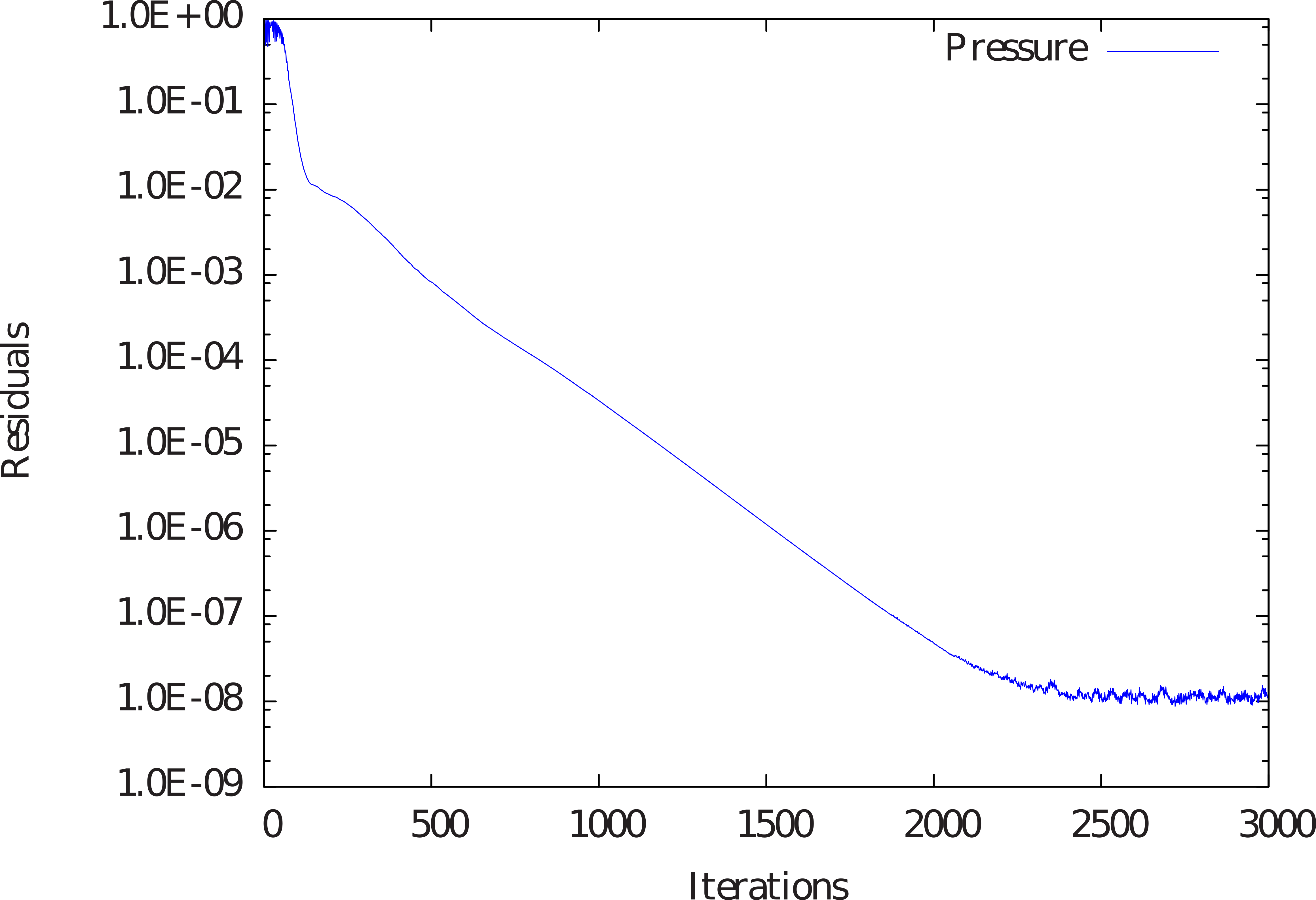
Figure 45 Convergence of pressure with respect to iterations
Results
The flow visualisation of velocity and pressure within the convex duct is presented here. In Figure 46 velocity magnitude and pressure are shown for SA model. Due to the convex bend, the thinning of the turbulent boundary layer occurs on the lower surface and the pressure decreases. Whereas the trends are opposite on the upper surface.
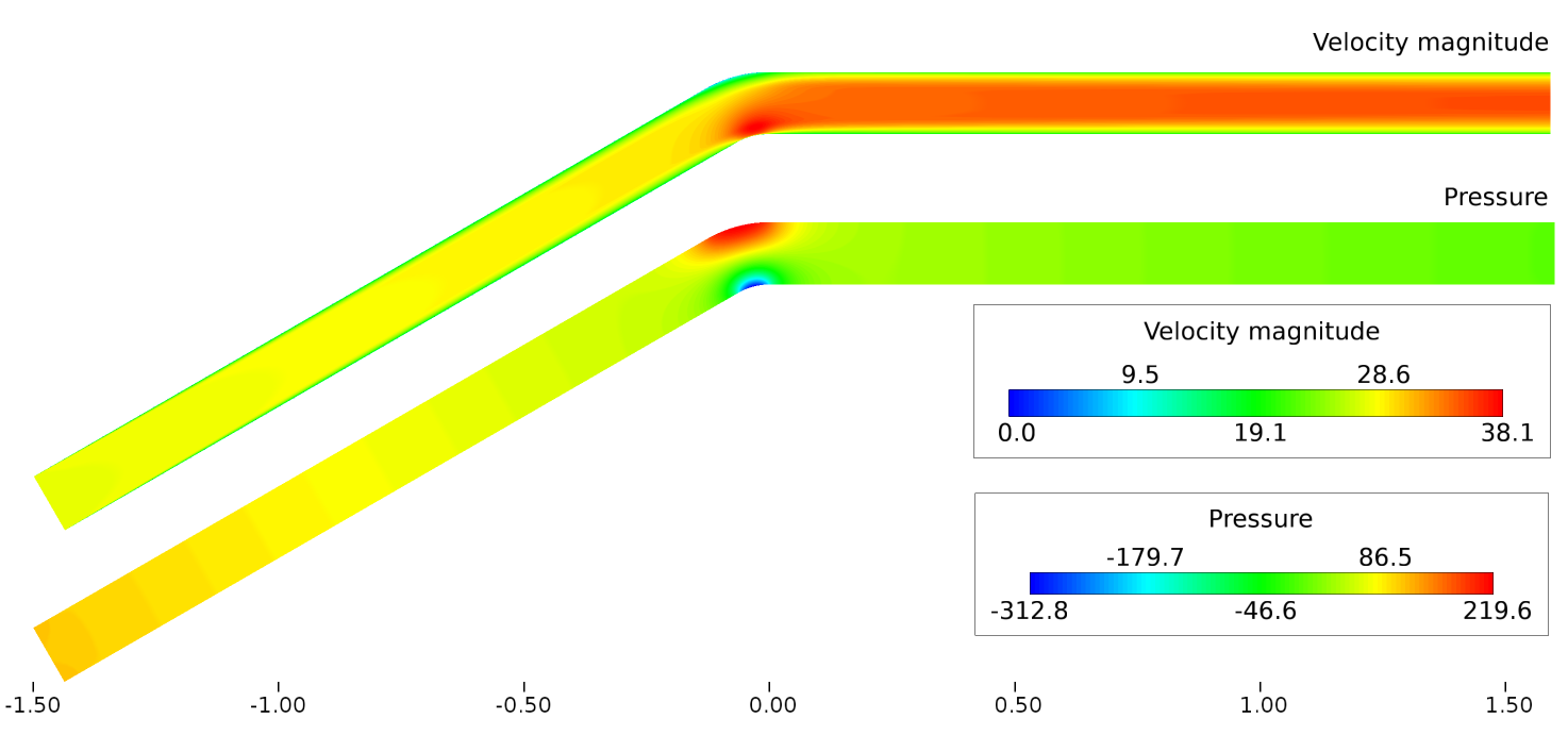
Figure 46 Velocity magnitude and pressure contours within the convex duct
Backward Facing Step
This tutorial focuses on the turbulent flow over a two-dimensional backward facing step using Caelus 9.04. In particular this tutorial emphasises the use of wall functions for a high \(y^+\) grid. The basic steps to set-up the directory structure, fluid properties, boundary conditions, turbulence properties etc will be discussed. Flow visualisation such as pressure and velocity contours within the separated region will be shown. With these steps in place, the user should be able to reproduce the tutorial accurately.
Objectives
Through this tutorial, the user will get familiar in setting up Caelus simulation for steady, turbulent, incompressible flow over a two-dimensional backward facing step with wall functions. Further, the velocity and pressure contours within the separated region will be highlighted. Following would be the steps that would be carried out.
- Background
A brief description about the problem
Geometry and freestream details
- Grid generation
Computational domain and boundary details
Computational grid generation
Exporting grid to Caelus
- Problem definition
Directory structure
Setting up boundary conditions, physical properties and control/solver attributes
- Execution of the solver
Monitoring the convergence
Writing the log files
- Results
Visualisation of flow over within the separated region
Pre-requisites
By now the user should be familiar with the Linux command line environment via a terminalor caelus-consolu (for Windows OS). The grid for this case can be obtained from the full working case directory shown below and was generated using Pointwise and appropriately converting it to Caelus format.
Background
Turbulent flow over a backward facing step is a classical configuration to examine steady separated flows. Here due to the presence of the step, the flow undergoes separation and the subsequent shear layer reattaches downstream forming a recirculation region. The thickness of the boundary layer at the lip of the step and the flow Reynolds number are important parameters that determines the length of separated region. A decrease in pressure or favourable pressure gradient in the immediate vicinity of the step is a classical behaviour that contributes to the increase in drag. The user is suggested to refer to the verification and validation of this case at Two-dimensional Backward Facing Step for more detailed analysis.
The schematic of the backward facing step is shown in Figure 47 in two-dimensions. A step height (H) of 1.0 m is used with a flow Reynolds number of 36000, which is based on the step height. Air is considered as a fluid with a freestream temperature of 298 K and the freestream velocity corresponds to U = 44.315 m/s. The user should note that the two-dimensional geometric plane considered is in \(x-z\) directions.
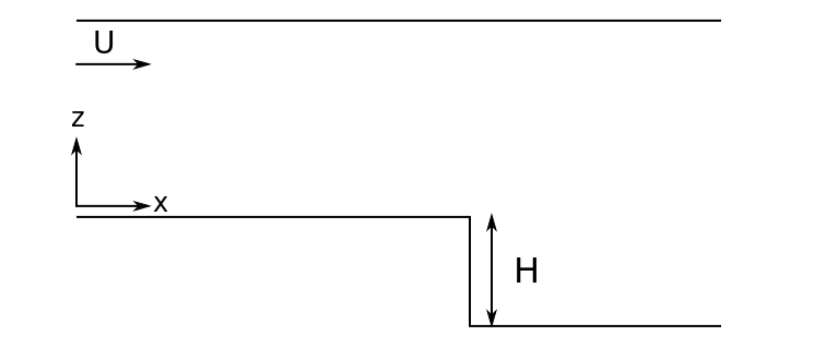
Figure 47 Schematic representation of the backward facing step
Freestream conditions are detailed in the below table
Fluid |
\(Re_H\) |
\(U~(m/s)\) |
\(p~(m^2/s^2)\) |
\(T~(K)\) |
\(\nu_\infty~(m^2/s)\) |
|---|---|---|---|---|---|
Air |
\(36000\) |
44.31525 |
\((0)\) Gauge |
298.330 |
\(1.230979\times10^{-3}\) |
Grid Generation
A fully structured gird is developed for this geometry and is converted to polyMesh format. The grid in polyMesh format can be found in the full working directory of this case at
/tutorials/incompressible/simpleSolver/ras/ACCM_backwardFacingStep2D/constant/polyMesh
The computational domain for the step is shown in Figure 48 which also highlights the boundary conditions used. The upstream flat plate extends for up to 110 step heights so that a fully turbulent boundary layer is ensured prior to the step at which the flow separates. Downstream of the step, the plate extends to 50 step heights giving sufficient length for the flow to reattach. The inlet and the outlet is placed as indicated in the Figure 48 and closely flows the experimental set-up. The velocity on the step surfaces is zero, wherein \(u,v,w = 0\) represented through a no-slip boundary.
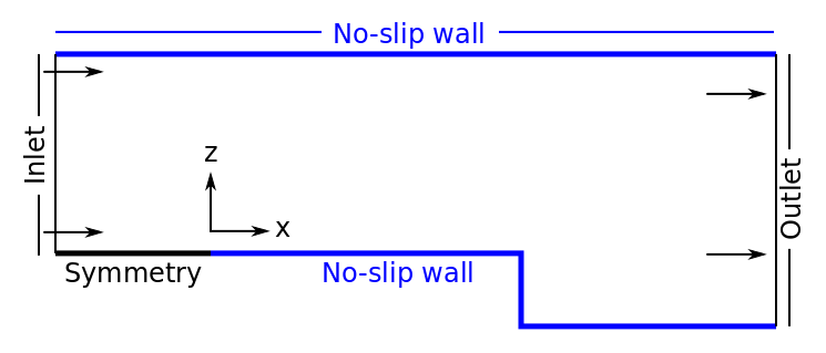
Figure 48 Computational domain of a 2D backward facing step
The grid in polyMesh is in three-dimensions, although the flow over the step is two-dimensional in nature. A one-cell thick grid normal to the flow plane (\(x-z\)) is therefore sufficient for Caelus to consider symmetry flow in the \(y\) direction. The two resulting planes that are in (\(x-z\)) direction need boundary conditions to be specified. Since the flow is assumed to be 2D, we do not need to solve the flow in the third-dimension and this can be easily achieved in Caelus by specifying empty boundary conditions for each of the two planes. This consequently treats the flow in :math`y` direction as symmetry.
Note
A velocity value of \(v=0\) needs to be specified at appropriate boundaries although no flow is solved in the \(y\) direction.
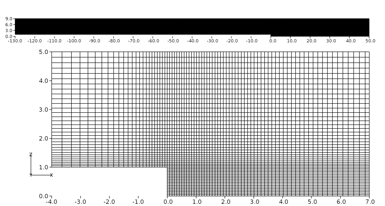
Figure 49 Computational grid of a 2D backward facing step in \(x-z\) plane
The 2D step grid in \(x-z\) plane is shown in figure %s:numref:t-step-grid-tutorials which has a total of 189 cells in the streamwise direction and 64 cells in the normal direction, with 20 cells representing the step height. As noted earlier, the grid is developed to use with wall functions and hence the \(y^+ \approx 30\) in this case.
Problem definition
This section details various steps needed to set-up the turbulent flow over a step. A full working case of this can be found in:
/tutorials/incompressible/simpleSolver/ras/ACCM_backwardFacingStep2D
However,the user is free to start the case setup from scratch consistent with the directory stucture discussed below.
Directory Structure
Note
All commands shown here are entered in a terminal window, unless otherwise mentioned
In order to set-up the problem Caelus requires time, constant and system sub-directories within the main working directory. Here, the simulation will be started at time t = 0 s, which requires a time sub-directory named 0.
The 0 sub-directory contains few additional files in which boundary conditions are specified. In the below table, the list of necessary files are provided based on the turbulence model chosen.
Parameter |
File name |
|---|---|
Pressure (\(p\)) |
|
Velocity (\(U\)) |
|
Turbulent viscosity (\(\nu\)) |
|
Turbulence field variable (\(\tilde{\nu}\)) |
|
Turbulent kinetic energy (\(k\)) |
|
Turbulent dissipation rate (\(\omega\)) |
|
Turbulent dissipation (\(\epsilon\)) |
|
In this tutorial we consider three turbulence models. They are Spalart-Allmaras (SA), \(k-\omega\) - Shear Stress Transport (\(\rm{SST}\)) and Realizable \(k-epsilon\) models. The content of the files listed above sets the dimensions, initialisation and boundary conditions to the defining problem, which also forms three principle entries required.
The user should note that Caelus is case sensitive and therefore the directory and file set-up should be identical to what is shown here.
Boundary Conditions and Solver Attributes
Boundary Conditions
Referring back to Figure 48, the following are the boundary conditions that will be specified:
- Inlet
Velocity: Fixed uniform velocity \(u = 44.31525~m/s\) in \(x\) direction
Pressure: Zero gradient
Turbulence:
Spalart–Allmaras (Fixed uniform values of \(\nu_{t~\infty}\) and \(\tilde{\nu}_{\infty}\) as given in Turbulence freestream conditions for SA model)
\(k-\omega~\rm{SST}\) (Fixed uniform values of \(k_{\infty}\), \(\omega_{\infty}\) and \(\nu_{t~\infty}\) as given in Turbulence freestream conditions for SA model)
Realizable \(k-\epsilon\) (Fixed uniform value of \(k_{\infty}\), \(\epsilon_{\infty}\) and \(\nu_{t_\infty}\) as given in Turbulent freestream conditions for Realizable k-\epsilon Model)
- Symmetry
Velocity: Symmetry
Pressure: Symmetry
Turbulence: Symmetry
- No-slip wall
Velocity: Fixed uniform velocity \(u, v, w = 0\)
Pressure: Zero gradient
Turbulence:
Spalart–Allmaras:
\(\nu_t\): type nutUWallFunction with a uniform value of \(\nu_t=0\)
\(\tilde{\nu}\): type fixedValue with a value of \(\tilde{\nu}=0\)
\(k-\omega~\rm{SST}\):
\(k\): type kqRWallFunction with a uniform value of \(k_{\infty}\)
\(\omega\): type omegaWallFunction with a uniform value of \(\omega_{\infty}\)
\(\nu_t\): type nutUWallFunction with a uniform value of \(\nu_t=0\)
Realizable \(k-\epsilon\):
\(k\): type kqRWallFunction with a uniform value of \(k_{\infty}\)
\(\epsilon\): type epsilonWallFunction with a uniform value of \(\epsilon=0\)
\(\nu_t\): type nutUWallFunction with a uniform value of \(\nu_t=0\)
- Outlet
Velocity: Zero gradient velocity
Pressure: Fixed uniform gauge pressure \(p = 0\)
Turbulence:
Spalart–Allmaras (Calculated \(\nu_{t}=0\) and Zero gradient \(\tilde{\nu}\))
\(k-\omega~\rm{SST}\) (Zero gradient \(k\) and \(\omega\); Calculated \(\nu_t=0\); )
Realizable \(k-\epsilon\) (Zero gradient \(k\) and \(\epsilon\); Calculated \(\nu_t=0\); )
- Initialisation
Velocity: Fixed uniform velocity \(u = 44.31525\) in \(x\) direction
Pressure: Zero Gauge pressure
Turbulence:
Spalart–Allmaras (Fixed uniform values of \(\nu_{t~\infty}\) and \(\tilde{\nu}_{\infty}\) as given in Turbulence freestream conditions for SA model)
\(k-\omega~\rm{SST}\) (Fixed uniform values of \(k_{\infty}\), \(\omega_{\infty}\) and \(\nu_{t~\infty}\) as given in Turbulence freestream conditions for SA model)
Realizable \(k-\epsilon\) (Fixed uniform values of \(k_{\infty}\), \(\epsilon_{\infty}\) and \(\nu_{t~\infty}\) as given in Turbulent freestream conditions for Realizable k-\epsilon Model)
First, the file p, shown below, contains initial and boundary conditions for pressure.
/*---------------------------------------------------------------------------*\
Caelus 9.04
 Web:      www.caelus-cml.com
\*---------------------------------------------------------------------------*/
FoamFile
{
    version     2.0;
    format      ascii;
    class       volScalarField;
    location    "0";
    object      p;
}
// * * * * * * * * * * * * * * * * * * * * * * * * * * * * * * * * * * * * * //

dimensions      [0 2 -2 0 0 0 0];

internalField   uniform 0;

boundaryField
{
    inlet
    {
        type            zeroGradient;
    }
    outlet
    {
        type            fixedValue;
        value           uniform 0;
    }
    symm-left
    {
        type            empty;
    }
    symm-right
    {
        type            empty;
    }
    top-wall
    {
        type            zeroGradient;
    }
    upstream
    {
        type            symmetryPlane;
    }
    wall
    {
        type            zeroGradient;
    }
}


// ************************************************************************* //
As can be noted from the above file, it begins with a dictionary named FoamFile which contains the standard set of keywords for version, format, location, class and object names. The explanation of the principle entries are as follows
dimensionis used to specify the physical dimensions of the pressure field. Here, pressure is defined in terms of kinematic pressure with the units (\(m^2/s^2\)) written as
[0 2 -2 0 0 0 0]
internalFieldis used to specify the initial conditions. It can be either uniform or non-uniform. Since we have a 0 initial uniform gauge pressure, the entry is
uniform 0;
boundaryFieldis used to specify the boundary conditions. In this case its the boundary conditions for pressure at all the boundary patches.
In the similar way, the file U is defined for velocity
/*---------------------------------------------------------------------------*\
Caelus 9.04
 Web:      www.caelus-cml.com
\*---------------------------------------------------------------------------*/
FoamFile
{
    version     2.0;
    format      ascii;
    class       volVectorField;
    location    "0";
    object      U;
}
// * * * * * * * * * * * * * * * * * * * * * * * * * * * * * * * * * * * * * //

dimensions      [0 1 -1 0 0 0 0];

internalField   uniform (44.31525 0 0);

boundaryField
{
    inlet
    {
        type            fixedValue;
        value           uniform (44.31525 0 0);
    }
    outlet
    {
        type            zeroGradient;
    }
    symm-left
    {
        type            empty;
    }
    symm-right
    {
        type            empty;
    }
    top-wall
    {
        type            noSlipWall;
    }
    upstream
    {
        type            symmetryPlane;
    }
    wall
    {
        type            noSlipWall;
    }
}


// ************************************************************************* //
The principle entries for velocity field are self-explanatory and the dimensions are typically for that of velocity with the units \(m/s\) ([0 1 -1 0 0 0 0]). Here, both initialisation and inlet have a uniform flow velocity specified with three velocity components. Therefore these should be set to uniform (44.31525 0 0); while the wall is given a no-slip condition.
The turbulent properties are also required to be specified at the boundary patches and these can be done similar to p and U. We have the file nut, which defines turbulent kinematic viscosity in the domain as follows
/*---------------------------------------------------------------------------*\
Caelus 9.04
 Web:      www.caelus-cml.com
\*---------------------------------------------------------------------------*/
FoamFile
{
    version     2.0;
    format      ascii;
    class       volScalarField;
    location    "0";
    object      nut;
}
// * * * * * * * * * * * * * * * * * * * * * * * * * * * * * * * * * * * * * //

dimensions      [0 2 -1 0 0 0 0];

internalField   uniform 0.09811;

boundaryField
{
    inlet
    {
        type            calculated;
        value           uniform 0.09811;
    }
    outlet
    {
        type            calculated;
        value           uniform 0;
    }
    symm-left
    {
        type            empty;
    }
    symm-right
    {
        type            empty;
    }
    top-wall
    {
        type            nutUWallFunction;
        Cmu             0.09;
        kappa           0.41;
        E               9.8;
        value           uniform 0;
    }
    upstream
    {
        type            symmetryPlane;
    }
    wall
    {
        type            nutUWallFunction;
        Cmu             0.09;
        kappa           0.41;
        E               9.8;
        value           uniform 0;
    }
}


// ************************************************************************* //
As noted above, the turbulent viscosity is specified as kinematic and therefore the units are in \(m^2/s\) ([0 2 -1 0 0 0 0]). The turbulent viscosity value at freestream, specified at inlet patch is calculated as detailed in Turbulence freestream conditions for SA model, Turbulent freestream conditions for k-\omega~\rm{SST} Model and Turbulent freestream conditions for Realizable k-\epsilon Model for SA, SST and RKE models respectively and is specified accordingly. The same value also goes for internalField.
The next turbulent property set is the nuTilda which is a turbulent field variable, specified to only SA model and has the same units ([0 2 -1 0 0 0 0]) as kinematic turbulent viscosity. Details pertaining to this are given in Turbulence freestream conditions for SA model. The following is the file nuTilda with the entries specified for the boundaryField are identical to that of turbulent kinematic viscosity explained above.
/*---------------------------------------------------------------------------*\
Caelus 9.04
 Web:      www.caelus-cml.com
\*---------------------------------------------------------------------------*/
FoamFile
{
    version     2.0;
    format      ascii;
    class       volScalarField;
    location    "0";
    object      nuTilda;
}
// * * * * * * * * * * * * * * * * * * * * * * * * * * * * * * * * * * * * * //

dimensions      [0 2 -1 0 0 0 0];

internalField   uniform 0.003692937;

boundaryField
{
    inlet
    {
        type            fixedValue;
        value           uniform 0.003692937;
    }
    outlet
    {
        type            zeroGradient;
    }
    symm-left
    {
        type            empty;
    }
    symm-right
    {
        type            empty;
    }
    top-wall
    {
        type            fixedValue;
        value           uniform 0;
    }
    upstream
    {
        type            symmetryPlane;
    }
    wall
    {
        type            fixedValue;
        value           uniform 0;
    }
}


// ************************************************************************* //
We can now proceed to the file k which is specific to both \(k-omega~\rm{SST}\) and Realizable \(k-epsilon\) models and represents turbulent kinetic energy.
/*---------------------------------------------------------------------------*\
Caelus 9.04
 Web:      www.caelus-cml.com
\*---------------------------------------------------------------------------*/
FoamFile
{
    version     2.0;
    format      ascii;
    class       volScalarField;
    location    "0";
    object      k;
}
// * * * * * * * * * * * * * * * * * * * * * * * * * * * * * * * * * * * * * //

dimensions      [0 2 -2 0 0 0 0];

internalField   uniform 0.2945755;

boundaryField
{
    inlet
    {
        type            fixedValue;
        value           uniform 0.2945755;
    }
    outlet
    {
        type            zeroGradient;
    }
    symm-left
    {
        type            empty;
    }
    symm-right
    {
        type            empty;
    }
    top-wall
    {
        type            kqRWallFunction;
        value           uniform 0.2945755;
    }
    upstream
    {
        type            symmetryPlane;
    }
    wall
    {
        type            kqRWallFunction;
        value           uniform 0.2945755;
    }
}


// ************************************************************************* //
The unit of kinetic energy is \(m^2/s^2\) and this is set in dimensions as [0 2 -2 0 0 0 0]. The value of \(k\) (refer Turbulent freestream conditions for k-\omega~\rm{SST} Model and Turbulent freestream conditions for Realizable k-\epsilon Model) needs to be specified for internalField, inlet and wall. Please note that for wall kqRWallFunction with values of freestream are required.
We now proceed to the file omega, specific to only \(k-\omega~\rm{SST}\) model and the value for this is evaluated as detailed in Turbulent freestream conditions for k-\omega~\rm{SST} Model
/*---------------------------------------------------------------------------*\
Caelus 9.04
 Web:      www.caelus-cml.com
\*---------------------------------------------------------------------------*/
FoamFile
{
    version     2.0;
    format      ascii;
    class       volScalarField;
    location    "0";
    object      omega;
}
// * * * * * * * * * * * * * * * * * * * * * * * * * * * * * * * * * * * * * //

dimensions      [0 0 -1 0 0 0 0];

internalField   uniform 97.37245;

boundaryField
{
    inlet
    {
        type            fixedValue;
        value           uniform 97.37245;
    }
    outlet
    {
        type            zeroGradient;
    }
    symm-left
    {
        type            empty;
    }
    symm-right
    {
        type            empty;
    }
    top-wall
    {
        type            omegaWallFunction;
        Cmu             0.09;
        kappa           0.41;
        E               9.8;
        beta1           0.075;
        value           uniform 97.37245;
    }
    upstream
    {
        type            symmetryPlane;
    }
    wall
    {
        type            omegaWallFunction;
        Cmu             0.09;
        kappa           0.41;
        E               9.8;
        beta1           0.075;
        value           uniform 97.37245;
    }
}


// ************************************************************************* //
The unit of specific rate of dissipation for \(\omega\) is \(1/s\) which is set in dimensions as [0 0 -1 0 0 0 0]. The internalField and inlet gets a fixedValue. Note that for wall boundaryField, we specify omegaWallFunction required for high \(y^+\).
The final file in this class is the epsilon, specific to only Realizable \(k-\epsilon\) model and the value for this is evaluated as detailed in Turbulent freestream conditions for Realizable k-\epsilon Model
/*---------------------------------------------------------------------------*\
Caelus 9.04
 Web:      www.caelus-cml.com
\*---------------------------------------------------------------------------*/
FoamFile
{
    version     2.0;
    format      ascii;
    class       volScalarField;
    location    "0";
    object      epsilon;
}
// * * * * * * * * * * * * * * * * * * * * * * * * * * * * * * * * * * * * * //

dimensions      [0 2 -3 0 0 0 0];

internalField   uniform 0.079598;

boundaryField
{
    inlet
    {
        type            fixedValue;
        value           uniform 0.079598;
    }
    outlet
    {
        type            zeroGradient;
    }
    symm-left
    {
        type            empty;
    }
    symm-right
    {
        type            empty;
    }
    top-wall
    {
        type            epsilonWallFunction;
        value           uniform 0;
    }
    upstream
    {
        type            symmetryPlane;
    }
    wall
    {
        type            epsilonWallFunction;
        value           uniform 0;
    }
}


// ************************************************************************* //
The unit of turbulent dissipation for \(\epsilon\) is \(m^2/s^3\) which is set in dimensions as [0 2 -3 0 0 0 0]. The internalField and inlet gets a fixedValue similar to \(\omega\). Note that for wall boundaryField, we specify epsilonWallFunction required for high \(y^+\).
Before proceeding to the next step, it is vital to ensure that the boundary conditions (inlet, outlet, wall, etc) added in the above files should be the grid boundary patches (surfaces) generated by grid generation tool and their names are identical. Additionally, the two boundaries \(x-z\) plane named here as symm-left and symm-right have empty boundary conditions which forces Caelus to assume the flow to be in two-dimensions. With this, the setting up of the boundary conditions are complete.
Grid file and Physical Properties
The files associated with the grid need to be placed in polyMesh sub-directory, which resides in the constant directory. We use identical grid for all the three turbulence simulation. In addition, the physical properties are specified in various different files present in the constant directory.
There are three files listed in addition to the polyMesh sub-directory. The first one, RASProperties in which the Reynolds-Average-Stress (RAS) model is specified, which is shown below. Please note that depending on the turbulence model you wish to run with, the line that corresponds to that specific model should be enabled.
/*-------------------------------------------------------------------------------*
Caelus 9.04
Web:   www.caelus-cml.com
\*------------------------------------------------------------------------------*/

FoamFile
{
	version			2.0;
	format			ascii;
	class			dictionary;
	location		"constant";
	object			RASProperties;
}

//--------------------------------------------------------------------------------

// For Spalarat-Alamaras Model, enable the below line
//RASModel				SpalartAllmaras;

// For k-omega SST Model, enable the below line
//RASModel				kOmegaSST;


// For Realizable k-epsilon Model, enable the below line
RASModel			realizableKE;

turbulence			on;

printCoeffs			on;
Second from the list is the transportProperties file, where laminar kinematic viscosity is specified as shown below
/*-------------------------------------------------------------------------------*
Caelus 9.04
Web:   www.caelus-cml.com
\*------------------------------------------------------------------------------*/
FoamFile
{
	version			2.0;
	format			ascii;
	class			dictionary;
	location		"constant";
	object			transportProperties;
}

//--------------------------------------------------------------------------------

transportModel			Newtonian;

nu				nu [0 2 -1 0 0 0 0] 1.230979E-3;

//Cross Power law and Bird-Carreau non-linear viscosity models
// ----------------------------------------------------------------------------
CrossPowerLawCoeffs
{
	nu0             	nu0 [0 2 -1 0 0 0 0] 1e-06;
	nuInf           	nuInf [0 2 -1 0 0 0 0] 1e-06;
	m               	m [0 0 1 0 0 0 0] 1;
	n               	n [0 0 0 0 0 0 0] 1;
}

BirdCarreauCoeffs
{
	nu0             	nu0 [0 2 -1 0 0 0 0] 1e-06;
	nuInf           	nuInf [0 2 -1 0 0 0 0] 1e-06;
	k               	k [0 0 1 0 0 0 0] 0;
	n               	n [0 0 0 0 0 0 0] 1;
}

//------------------------------------------------------------------------------
The viscous behaviour is modelled as Newtonian and hence the keyword Newtonian is used for the transportModel and the molecular (laminar) kinematic viscosity (\(nu\)) is given having the units \(m^2/s\) ([0 2 -1 0 0 0 0]).
The final file in this class is the turbulenceProperties file, which sets the simulationType to RASModel. Here, SA, \(k-\omega~\rm{SST}\) and Realizable \(k-\epsilon\) are classified as Reynolds Average Stress (RAS) models.
/*-------------------------------------------------------------------------------*
Caelus 9.04
Web:   www.caelus-cml.com
\*------------------------------------------------------------------------------*/
FoamFile
{

	version			2.0;
	format			ascii;
	class			dictionary;
	location		"constant";
	object			turbulenceProperties;
}

//-----------------------------------------------------------------------------

simulationType			RASModel;

//-----------------------------------------------------------------------------
Controls and Solver Attributes
This section details the files required to control the simulation, discretization methods and linear solvers. These files are to be placed in the system directory. First, navigate to the system directory
The following is the controlDict file,
/*-------------------------------------------------------------------------------*
Caelus 9.04
Web:   www.caelus-cml.com
\*------------------------------------------------------------------------------*/

FoamFile
{
	version			2.0;
	format			ascii;
	class			dictionary;
	location		"system";
	object			controlDict;
}

//--------------------------------------------------------------------------------

application			simpleSolver;

startFrom			startTime;

startTime			0;

stopAt				endTime;

endTime				10000;

deltaT				1.0;

writeControl			runTime;

writeInterval			500;

purgeWrite			0;

writeFormat			ascii;

writePrecision			12;

writeCompression 		true;

timeFormat			general;

timePrecision			12;

runTimeModifiable		true;

//-------------------------------------------------------------------------------

// Function Objects to obtain forces

/*functions
{
	forces
	{
		type		forces;

        functionObjectLibs 	("libforces.so");
        patches     		( wall );
        CofR      		(0 0 0);
        rhoName         	rhoInf;
        rhoInf          	15.13009E-3;
        outputControl   	timeStep;
        outputInterval  	100;
     }
}
Here, simpleSolver is used and the simulation begins at t = 0 s. This now explains the logical need for having a 0 directory where the data files are read at the beginning of the run, which is t = 0 s in this case. Therefore, the keyword startFrom is set to startTime, where startTime is set to 0. The simulation would be carried out as steady-state and therefore we require to specify the total number of iterations as a keyword for endTime. Via the writeControl and writeInterval keywords, the solution intervals at which they are saved can be specified. Also note that a function object to obtain the force over the wall (step surface) for every 100 iterations is included. In order to obtain this, a freestream density (rhoInf) need to be specified.
The discretization schemes for the finite volume discretization that will be used should be set through the fvSchemes file show below
/*-------------------------------------------------------------------------------*
Caelus 9.04
Web:   www.caelus-cml.com
\*------------------------------------------------------------------------------*/

FoamFile
{
	version				2.0;
	format				ascii;
	class				dictionary;
	object				fvSchemes;
}

//------------------------------------------------------------------------------

ddtSchemes
{
	default				steadyState;
}

gradSchemes
{
	default				Gauss	linear;
	grad(p)				Gauss	linear;
	grad(U)				Gauss	linear;
}

divSchemes
{
	default				none;
	div(phi,U)			Gauss	linearUpwind 	grad(U);
	div(phi,nuTilda)		Gauss	upwind;		                    // Will be used for S-A model only
	div(phi,k)      		Gauss	upwind; 	                    // will be used for k-epsilon & k-omega only
	div(phi,omega)  		Gauss 	upwind;				// Will be used for k-omega model only
	div(phi,epsilon)	  	Gauss 	upwind;
	div((nuEff*dev(T(grad(U)))))	Gauss   linear;
	div(phi,symm(grad(U)))		Gauss	linear;				// Will be used for S-A-Curvature-corr only
}

laplacianSchemes
{
	default				none;
	laplacian(nu,U)			Gauss 	linear	corrected;
	laplacian(nuEff,U)		Gauss 	linear	corrected;
	laplacian(DnuTildaEff,nuTilda)  Gauss 	linear 	corrected; // Will be used for S-A model only
	laplacian(DkEff,k) 		Gauss 	linear 	corrected; // Will be used for k-omega & k-omega only
	laplacian(DomegaEff,omega) 	Gauss 	linear 	corrected; // Will be used for k-omega model only
	laplacian(DepsilonEff,epsilon)	Gauss 	linear 	corrected;
	laplacian(rAUf,p)		Gauss 	linear 	corrected;
	laplacian(1,p)  		Gauss 	linear 	corrected;
}

interpolationSchemes
{
	default				linear;
	interpolate(HbyA)		linear;
}

snGradschemes
{
	default				corrected;
}


//--------------------------------------------------------------------------------
The linear solver controls and tolerances are set in fvSolution as given below
/*-------------------------------------------------------------------------------*
Caelus 9.04
Web:   www.caelus-cml.com
\*------------------------------------------------------------------------------*/
FoamFile
{
        version                         2.0;
        format                          ascii;
        class                           dictionary;
        location                        "system";
        object                          fvSolution;
}

//------------------------------------------------------------------------------

solvers
{
        p
        {
            solver                      PCG;
            preconditioner              SSGS;
            tolerance                   1e-8;
            relTol                      0.01;
        }
        U
        {
            solver                      PBiCGStab;
            preconditioner              USGS;
            tolerance                   1e-7;
            relTol                      0.01;
        }

        "(k|omega|nuTilda|epsilon)"
        {
            solver                      PBiCGStab;
            preconditioner              USGS;
            tolerance                   1e-08;
            relTol                      0;
        }
}

SIMPLE
{
        nNonOrthogonalCorrectors        1;
        pRefCell                        0;
        pRefValue                       0;
}

relaxationFactors
{
    	p                               0.3;
    	U                               0.3;
        nuTilda                         0.5;
        k                               0.5;
        omega                           0.5;
        epsilon                         0.5;
}
The user should now take a note that in the fvSolution file, different linear solvers are used to solve for velocity, pressure and turbulence quantities. We also set the nNonOrthogonalCorrectors to 1 for this case. To ensure the stability of the solution, the relaxation is set to primary and turbulent variables. The relTol is not set to 0 unlike a time-accurate set-up as we are solving for a steady-state solution and a very low (\(\approx 0\)) tolerance at every iteration is unnecessary. Since the entire system of equations converge to a global set tolerance the convergence would occur as the solution progresses to a steady state.
With this, the set-up of the directory structure with all the relevant files are complete. This can be verified again by issuing the following command and the directory tree should appear identical to the one shown below
cd my-turbulent-step/
tree
.
├── 0
│   ├── epsilon
│   ├── k
│   ├── nut
│   ├── nuTilda
│   ├── omega
│   ├── p
│   └── U
├── constant
│   ├── polyMesh
│   │   ├── boundary
│   │   ├── faces
│   │   ├── neighbour
│   │   ├── owner
│   │   └── points
│   ├── RASProperties
│   ├── transportProperties
│   └── turbulenceProperties
└── system
    ├── controlDict
    ├── fvSchemes
    └── fvSolution
Execution of the solver
Prior to the execution of the solver, it is important to renumber and to carry out a quality check on the grid/mesh. Renumbering reduces the bandwidth whereas the quality check shows the mesh statistics. These two can be performed by executing the following commands from the top working directory
caelus run -- renumberMesh -overwrite
caelus run -- checkMesh
When the renumberMesh is performed, the user should take note of the bandwidth before and after the mesh renumbering. In a similar manner, when the checkMesh is performed, the mesh statistics are shown as below
/*---------------------------------------------------------------------------*\
 Caelus 8.04
 Web:      www.caelus-cml.com
\*---------------------------------------------------------------------------*/

Checking geometry...
    Overall domain bounding box (-130 0 0) (50 1 9)
    Mesh (non-empty, non-wedge) directions (1 0 1)
    Mesh (non-empty) directions (1 0 1)
    All edges aligned with or perpendicular to non-empty directions.
    Boundary openness (7.60426729195e-19 -3.46752522136e-15 6.3479100872e-18) OK.
    Max cell openness = 2.1851506874e-16 OK.
    Max aspect ratio = 205.17630165 OK.
    Minimum face area = 0.00417125. Maximum face area = 10.4153124857.  Face area magnitudes OK.
    Min volume = 0.00417125. Max volume = 1.987102972.  Total volume = 1490.  Cell volumes OK.
    Mesh non-orthogonality Max: 12.1317921302 average: 0.100202600449
    Non-orthogonality check OK.
    Face pyramids OK.
    Mesh skewness Max: 0.00821683161155 average: 8.01613031841e-06 OK.
    Coupled point location match (average 0) OK.

Mesh OK.

End
At this stage, the solver can be executed from the top directory using the following command
caelus run -l my-turbulent-step.log -- simpleSolver
The log file can be further processed to look at the convergence history and this can be done as follows
caelus logs -w my-turbulent-step.log
The caelus-plotResiduals -l allows you to look at the convergence of various variables with respect to the number of iterations carried out and is shown in Figure 50.
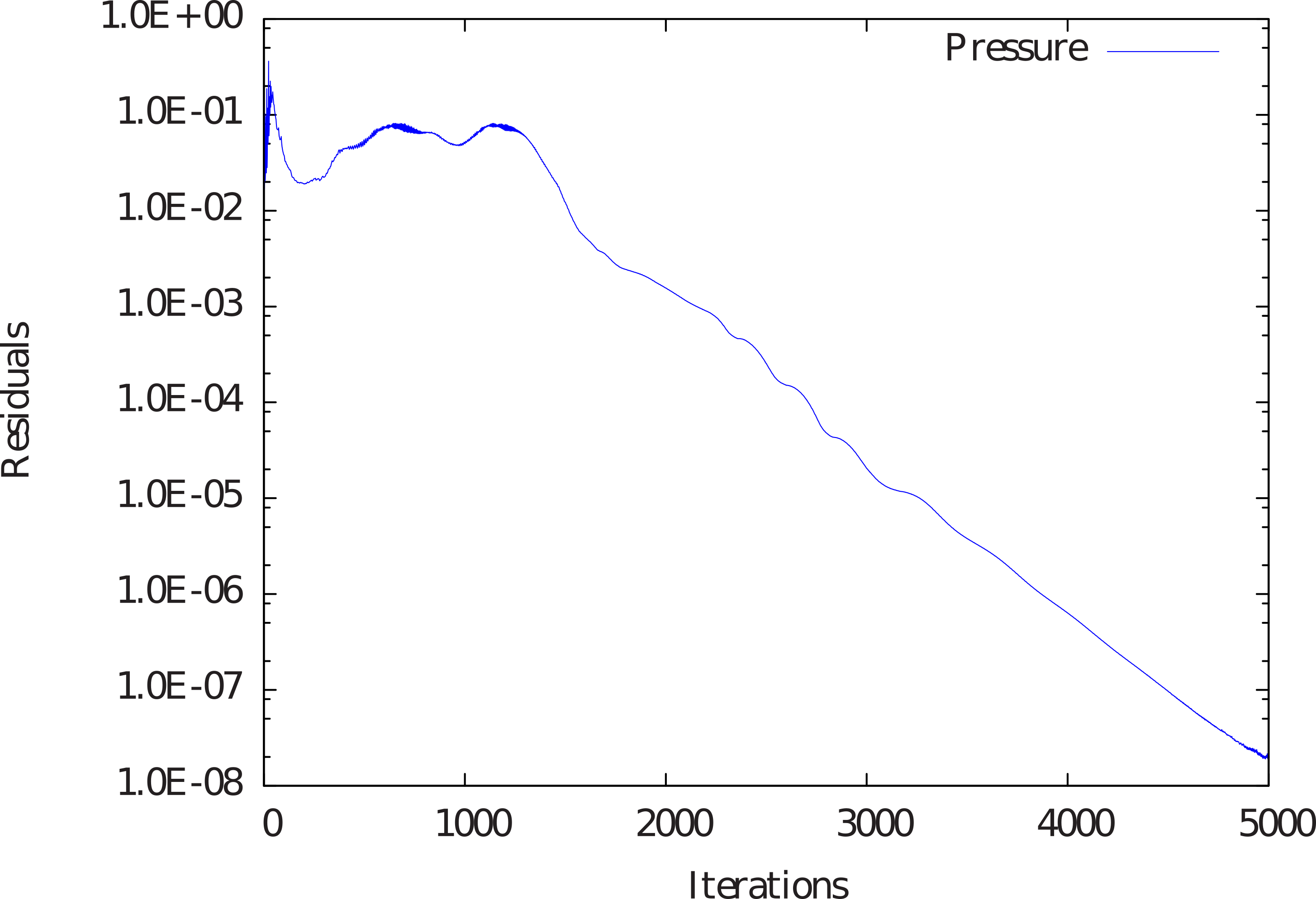
Figure 50 Convergence of pressure with respect to iterations
Results
The flow within the separated region is visualised here through the velocity and pressure contours. In Figure 51 velocity magnitude and pressure contours are shown for SA model. Immediate downstream of the step a decrease in pressure is seen followed by an increases as the shear layer reattaches to the step. This is consistent with the formation of a low velocity recirculating region behind the step.
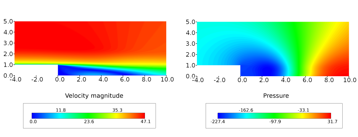
Figure 51 Velocity magnitude and pressure contours over the backward facing step